Discussion

Key findings:

             My project leveraged the Cleveland and VA Long Beach datasets, in the “Heart Disease” database, which was donated to the UCI Machine Learning Repository to explore the binary classification of heart disease presence, using the available demographic and clinical features. Through exploratory data analysis (EDA), data cleaning, transformation experiments, and model evaluation, several critical insights emerged. Transformation 2, which included logarithmic transformations for skewed features, a squared transformation for maximum heart rate, and the creation of a combined feature (old peak and slope), was identified as the most effective preprocessing strategy. This approach enhanced feature stability and predictive accuracy on the Cleveland dataset and was subsequently applied to the VA Long Beach dataset to assess regional generalizability.

The Random Forest Classifier for Transformation 2 consistently outperformed other models in terms of prediction accuracy and robustness across multiple train-test splits. On the Cleveland dataset, the Random Forest Classifier achieved an accuracy of 83.33%, with balanced precision (85.56%) and recall (83.33%), supported by consistent cross-validation performance. Applied to the VA Long Beach dataset, the unoptimized Random Forest Classifier demonstrated a performance with an accuracy of 82.5%, precision of 80%, and recall of 40% for the minority class. Unlike its optimized counterpart, this configuration effectively mitigated the neglect of minority class predictions, striking a better balance between the classes.

While the Random Forest Classifier outperformed the ASCVD risk score on average across both datasets, achieving higher accuracy and F1 scores, it did not resolve variability in female subgroup predictions. On the Cleveland dataset, the ASCVD score achieved an AUC-ROC of 78.08% for females compared to 68.87% for males, and the Random Forest model exhibited similar imbalances. Female recall for the ASCVD was higher (88.89%) but precision was considerably lower (48.88%), resulting in a less balanced F1 score (62.87%) compared to males (72.73%). On the VA Long Beach dataset, the ASCVD score achieved strong recall (93.75%) but limited discriminatory power, with an AUC-ROC of 60.98%. The lack of sufficient female representation in the VA Long Beach dataset precluded any sex-specific analysis, underscoring the importance of diverse and balanced datasets.

Gender-based analysis on the Cleveland dataset revealed clear disparities in machine learning model performance with the Random Forest Classifier. While the model achieved high overall accuracy and precision; the model demonstrated considerably lower recall for female patients with heart disease (0.67). This variability indicates that the model, while improving overall performance compared to the ASCVD score, did not effectively address gender-specific prediction inconsistencies. Features such as Oldpeak and slope emerged as strong indicators of heart disease presence, whereas weaker relationships were observed for cholesterol and fasting blood sugar, suggesting limited predictive value for these variables within these datasets.

In conclusion, the Random Forest Classifier demonstrated superior average performance compared to the ASCVD risk score but fell short of addressing variability in female subgroup predictions. These findings highlight the importance of future work to explore gender-specific adjustments and strategies for achieving equitable performance across demographic groups, while also emphasizing the need for diverse datasets to enhance generalizability.

Regional generalizability

VA Long Beach models with optimized parameters highlight a few possible implications. Parameter optimization of the Random Forest Classifier, while improving the overall accuracy, had significant drawbacks when applied to a dataset with an imbalanced class distribution. The optimized model prioritized the majority class, resulting in a complete inability to predict any instances of the minority class (those with heart disease). This led to a recall of 0% for the minority class, effectively excluding it from the model’s predictions. Although overall accuracy increased, this came at the cost of fairness and utility, as the model failed to capture critical instances of the minority class. These findings highlight that, in the case of the Random Forest Classifier, parameter optimization compromised the model’s balance, favoring the majority class performance while neglecting the minority class.

            The comparison between the Cleveland and VA Long Beach models without optimized parameters further highlights two possible implications: optimized parameters can overgeneralize for the majority class, or they may reduce the model’s ability to classify effectively across regions. These potential drawbacks are particularly obscured by the small number of patients in the minority class (those without heart disease) in the VA Long Beach dataset, which makes it challenging to draw definitive conclusions.

Without optimization, the Random Forest Classifier still achieved balanced performance for the minority class on the Cleveland dataset, while still maintaining reasonable performance for the VA Long Beach dataset. However, with optimized parameters, the VA Long Beach model completely failed to predict any instances of the minority class, suggesting that the optimization may have tailored the model too closely to the majority class, resulting in overgeneralization.

These outcomes suggest that the small sample size of the minority class amplifies the difficulty in determining whether the reduced performance is due to overgeneralization for the majority class or a lack of adaptability across regions. This underscores the importance of balancing datasets and carefully evaluating the impact of optimization on both regional performance and minority class predictions.

Sex-specific performance summary

            The model assessing the male population achieved an accuracy of 78.05% and an F1-score of 78.31%. For class 0 (no heart disease), it recorded a precision of 68%, recall of 81%, and an F1-score of 74%. For class 1 (heart disease), the model demonstrated a higher precision of 86% but a lower recall of 76%, resulting in an F1-score of 81%. The overall weighted averages for precision, recall, and F1-score were 80%, 78%, and 78%, respectively, reflecting moderately balanced performance on the male population. In contrast, the model applied to the female population exhibited higher overall accuracy (94.74%) and F1-score (94%). The precision for class 0 was higher (94% compared to 67% in the male model), the recall for class 0 was significantly higher as well at 100%, surpassing the male model’s recall of 81%. For class 1, the female model achieved perfect precision (100%) but a lower recall of 67%, compared to the male model’s recall of 76%.

These results highlight distinct performance differences between the male and female subpopulations. The model demonstrated better overall accuracy and precision for the female population, but its ability to detect heart disease cases (class 1) was slightly lower in recall compared to the male population. Conversely, the male model exhibited a more balanced trade-off between precision and recall for class 1 but at the cost of a higher false positive rate. These findings underscore the need for additional tuning to ensure the model performs consistently across gender-specific groups, avoiding potential biases in prediction outcomes.

Data limitations

            Due to the limitations of the Cleveland data, with the male test set comprising 41 samples and the female test set comprising only 19 samples, I am unable to perform cross-validation for these subsets. This restriction limits the ability to thoroughly assess model generalizability and robustness across gender-specific groups. As a result, the interpretation of the results must be approached with caution, as the insights drawn may not fully capture the broader performance trends for male and female populations.

The VA Long Beach dataset had significant limitations that must be addressed. One key issue is the severe gender imbalance, with only approximately 6 females included in the dataset. This small number makes it impossible to test the model by gender, as there are insufficient entries to draw any meaningful conclusions for female patients.

Additionally, the dataset suffers from a pronounced class imbalance, with most instances representing individuals with heart disease. This imbalance introduces challenges for the model, as there is limited data available to effectively train the minority class (individuals without heart disease). As a result, there is a strong expectation of underfitting for the minority class, where the model may fail to accurately predict or generalize for these cases.

Another critical issue is the missing data. Columns such as “ca” (99% missing values) and “thal” (83% missing values) have so few valid entries that they needed to be removed from the analysis.

To ensure a fair comparison when evaluating models, I had to create modified Cleveland models for comparison. This was done by removing the “ca” and “thal” columns, aligning the feature set with the limitations of this dataset. This approach allowed for a slightly more balanced evaluation when comparing the models trained on the Cleveland dataset to the Long Beach Models.

Lastly, The ASCVD (Atherosclerotic Cardiovascular Disease) Risk Calculator was applied to both the Cleveland and VA Long Beach datasets to estimate the 10-year cardiovascular risk for individual patients. However, due to missing or unavailable data, proxies were used to ensure compatibility with the ASCVD model. HDL cholesterol was assigned a placeholder value of 50, and ethnicity was uniformly set to non-Black (isBlack = False) because explicit data on this characteristic was not available. Hypertension status was derived from systolic blood pressure (SBP) values, with readings of 130 or higher classified as hypertensive. Diabetes status was inferred from fasting blood sugar (fbs), with values over 120 converted into a boolean indicator (diabetic = True). Smoking status was approximated using exercise-induced angina (exang), with the absence of angina interpreted as non-smoking status (False).

While these proxies enabled the datasets to be used for ASCVD risk estimation, they introduced approximations that deviate from the precise inputs required by the ASCVD model. Consequently, the calculated risk scores are not pure ASCVD scores, but rather adapted estimates. This reliance on proxies adds a layer of uncertainty to the analysis and necessitates cautious interpretation of the results.

Future directions

My research highlighted several areas for improvement and exploration in future research. After evaluating the datasets and outcomes, it became evident that a more effective approach might involve transitioning from binary classification to multilabel classification. Specifically, this approach could predict varying levels of heart disease severity rather than focusing solely on the binary presence or absence of the condition. This shift in focus is motivated by the observation that, aside from the Cleveland dataset, the other cities’ datasets predominantly consist of patients with some degree of heart disease. The relative scarcity of individuals without heart disease in these datasets diminishes the utility of binary classification and underscores the potential for a more nuanced multilabel approach.

Additionally, my research revealed a significant gender imbalance in the datasets, with fewer females represented compared to males. This raises critical questions about whether this disparity reflects sampling bias or is indicative of real-world clinical trends. Considering that cardiovascular disease is a leading cause of death among women, it is essential to investigate why females may be underrepresented in these datasets. Future research should aim to address this imbalance, ensuring equitable representation to enhance the generalizability and fairness of predictive models.

Incorporating these changes, future studies could develop more accurate and reproducible models that account for demographic disparities and focus on the varying levels of heart disease severity. This approach would not only provide richer clinical insights but also foster more inclusive and accurate models capable of addressing the diverse needs of populations affected by cardiovascular disease.

Atherosclerotic Cardiovascular Disease Risk Calculation on Cleveland Dataset

The 2013 ASCVD (Atherosclerotic Cardiovascular Disease) risk score was evaluated on the Cleveland dataset, yielding key performance metrics. The score achieved an accuracy of 69.64%, indicating that approximately 70% of predictions matched actual outcomes. Precision was 63.58%, reflecting the proportion of correctly identified positive cases among all predicted positives, while recall was 79.14%, demonstrating the model’s ability to capture most actual positive cases. The F1 score, balancing precision and recall, was 70.51%, signifying a moderate trade-off between the two. Additionally, the AUC-ROC score of 70.36% suggests a fair level of discriminatory ability between positive and negative cases. These results indicate that the 2013 ASCVD risk score provides reasonable predictive performance for the Cleveland dataset, with notable strengths in recall but areas for improvement in precision and overall accuracy.

Female

Male

Performance Comparison

The performance comparison between male and female subgroups reveals notable differences, particularly in the variability of scores for the female group. For females, the model achieved an accuracy of 73.19%, slightly higher than the accuracy of 69.67% observed for males. However, the precision for females was lower at 48.88% compared to 68.75% for males, indicating that the model was less reliable in identifying true positives among predicted positives for the female subgroup. Conversely, the recall for females was significantly higher at 88.89%, compared to 77.19% for males, suggesting that the model was more effective in identifying actual positive cases among females

The F1 score, which balances precision and recall, highlights the disparity between the subgroups. Females achieved an F1 score of 62.87%, reflecting the impact of lower precision despite high recall, whereas males had a more balanced F1 score of 72.73%. The AUC-ROC scores further emphasize this difference, with females achieving 78.08% compared to 68.87% for males, indicating better overall discrimination for the female subgroup.

The wide variability in the scores for the female group, particularly the sharp contrast between high recall and low precision, underscores potential challenges in the model’s consistency when applied to different demographic subgroups. This variability suggests that further optimization or subgroup-specific adjustments may be necessary to ensure more balanced and equitable performance across genders.

Atherosclerotic Cardiovascular Disease Risk Calculation on VA Long Beach Dataset

The 2013 ASCVD (Atherosclerotic Cardiovascular Disease) risk score was evaluated on the VA Long Beach dataset, achieving an accuracy of 76.82%, indicating that over three-quarters of the predictions aligned with the actual outcomes. The precision of 78.95% highlights the model’s reliability in identifying true positives among predicted positives, while the recall of 93.75% demonstrates its ability to effectively detect the majority of actual positive cases. The F1 score, balancing precision and recall, was 85.71%, reflecting robust overall performance. However, the AUC-ROC score of 60.98% suggests limited discriminatory power between positive and negative classes, indicating room for improvement in distinguishing cases.

It is important to note that due to the small number of females in the VA Long Beach dataset, a sex-specific analysis was not feasible. This limitation restricts the ability to assess the model’s performance across different demographic subgroups and emphasizes the need for more diverse and balanced datasets in future analyses.

Is the Best Performing Models More Effective for Male vs. Female Population?

The highest-performing models were identified in Experiment 2, showcasing robust predictive capabilities. The Random Forest classifier emerged as the top performer, achieving a mean accuracy of 88.33%, a mean precision of 91.79%, a mean recall of 82.00%, and a mean F1-score of 83.67%. This model was tested separately on male and female populations to analyze gender-specific performance variations.

Random Forest Classifier test with optimized parameters for female population: transformation 2.

The model achieved an overall accuracy of 94.74% on the female test set, with a macro-average F1-score of 83% and a weighted average F1-score of 94%. It demonstrated strong performance in identifying individuals without heart disease (class 0), achieving a precision of 94%, a recall of 100%, and an F1-score of 97%. However, the performance for individuals with heart disease (class 1) was considerably weaker, with a recall of only 67%, indicating that the model struggled to identify all positive cases accurately. While the precision for class 1 was 100%, the low recall highlights a significant imbalance in the model’s ability to predict outcomes for this group.

Due to the limited sample size of the female test set (19 samples) and the inability to perform cross-validation, it is not possible to directly assess overfitting. However, the high accuracy and F1-scores, combined with the disproportionately low recall for class 1, suggest that the model may be overfitting to the test data, particularly favoring class 0. These results underscore the need for further data and evaluation to ensure the model’s generalizability and balanced performance across all classes.

Random Forest Classifier test with optimized parameters for male population: transformation 2.

The model assessing the male population achieved an accuracy of 78.05% and an F1-score of 78.31%. For class 0 (no heart disease), it recorded a precision of 67%, recall of 88%, and an F1-score of 76%. For class 1 (heart disease), the model demonstrated a higher precision of 90% but a lower recall of 72%, resulting in an F1-score of 80%. The overall weighted averages for precision, recall, and F1-score were 81%, 78%, and 78%, respectively, reflecting moderately balanced performance on the male population.

In contrast, the model applied to the female population exhibited higher overall accuracy (94.74%) and F1-score (94%). While the precision for class 0 was slightly lower (94% compared to 67% in the male model), the recall for class 0 was significantly higher at 100%, surpassing the male model’s recall of 88%. For class 1, the female model achieved perfect precision (100%) but a lower recall of 67%, compared to the male model’s recall of 72%.

Comparison of Performance.

            The model assessing the male population achieved an accuracy of 78.05% and an F1-score of 78.31%. For class 0 (no heart disease), it recorded a precision of 67%, recall of 88%, and an F1-score of 76%. For class 1 (heart disease), the model demonstrated a higher precision of 90% but a lower recall of 72%, resulting in an F1-score of 80%. The overall weighted averages for precision, recall, and F1-score were 81%, 78%, and 78%, respectively, reflecting moderately balanced performance on the male population.

In contrast, the model applied to the female population exhibited higher overall accuracy (94.74%) and F1-score (94%). While the precision for class 0 was lower (94% compared to 67% in the male model), the recall for class 0 was significantly higher at 100%, surpassing the male model’s recall of 88%. For class 1, the female model achieved perfect precision (100%) but a lower recall of 67%, compared to the male model’s recall of 72%.

These results highlight distinct performance differences between the male and female subpopulations. The model demonstrated better overall accuracy and precision for the female population, but its ability to detect heart disease cases (class 1) was slightly lower in recall compared to the male population. Conversely, the male model exhibited a more balanced trade-off between precision and recall for class 1 but at the cost of a higher false positive rate. These findings underscore the need for additional tuning to ensure the model performs consistently across gender-specific groups, avoiding potential biases in prediction outcomes.

Optimizing Feature Engineering

In this third experiment, the focus is on enhancing the feature engineering component to improve model performance through targeted transformations. The following transformations were applied: (1) a logarithmic transformation for Resting Blood Pressure (trestbps) and Cholesterol (chol) to reduce skewness and stabilize variance; (2) a squared transformation of Maximum Heart Rate (thalach), which emphasizes the importance of higher values in this feature; and (3) the creation of a combined feature using Oldpeak and Slope, aimed at capturing their interaction and improving predictive power. Additionally, gender-based feature engineering was introduced to account for potential differences across genders.

Gender Based Feature Engineering:

            This process introduced new features to capture gender-specific patterns within the dataset. Six gender-specific features were implemented to identify and capture gender-related patterns within the dataset, enhancing the model’s ability to discern variations between male and female groups. The first feature, `thalach_norm_gender`, normalizes the maximum heart rate achieved (`thalach`) within each gender group by dividing individual values by the mean `thalach` for that group. Similarly, the second feature, `chol_norm_gender`, normalizes serum cholesterol (`chol`) values by dividing them by the mean cholesterol value for the respective gender.

Additionally, gender-specific indicators were introduced to flag deviations from the typical range within each gender group. The feature `thalach_above_median_gender` is a binary indicator (0 or 1) that signals whether a person’s `thalach` exceeds the median `thalach` value for their gender. In parallel, `chol_above_median_gender` functions as a binary indicator, identifying individuals whose `chol` values surpass the median cholesterol level within their gender group. Together, these features provide a nuanced representation of gender-specific patterns, potentially improving the predictive performance of models trained on the dataset.

Random Forest Classifier.

The Random Forest classifier, implemented without parameter optimization, demonstrated an accuracy of 83.33%, indicating that the majority of predictions were correct. The precision of 83.33% suggests the model was effective in minimizing false positives, while the recall, also at 83.33%, indicates a balanced ability to identify true positives. The F1-score of 83.28% reflects the overall mean of precision and recall, showcasing strong model performance. The confusion matrix shows the model correctly classified 28 true negatives and 22 true positives, with 4 false positives and 6 false negatives.

Cross-validation results further evaluated the model’s consistency, with a mean accuracy of 78.33%, precision of 75.19%, recall of 72.29%, and F1-score of 72.15%.

Grid Search Overview.

The grid search process evaluated 80 different hyperparameter combinations across three folds, resulting in 240 total model fits. The best parameters identified were a `max_depth` of 3, `n_estimators` of 50, and a `random_state` of 2024. With these hyperparameters, the model achieved a best cross-validated F1-weighted score of 0.8488, indicating improved balance between precision and recall compared to the default settings. This highlights the positive impact of hyperparameter tuning on the Random Forest model’s performance.

Application of Optimized Parameters for Random Forest Classifier.

The application of optimized parameters to the Random Forest classifier resulted in an accuracy of 83.33%, consistent with the unoptimized model. The precision improved slightly to 84.38%, while recall remained at 83.33%. The F1-score of 83.18% reflects balanced performance but shows a minor decrease compared to previous results. The confusion matrix indicates 29 true negatives, 21 true positives, 3 false positives, and 7 false negatives.

Cross-validation results reveal a mean accuracy of 78.33%, mean precision of 74.17%, mean recall of 76.14%, and mean F1-score of 72.42%. While these results are reasonable, there is a noticeable overall drop in performance metrics compared to prior experiments. This suggests that the optimized parameters, though improving precision, might have introduced trade-offs that slightly reduced the model’s ability to generalize consistently across folds. Further fine-tuning or exploration of different parameter combinations may be needed to enhance performance.

XGBoost Classifier.

The XGBoost classifier, run without optimized parameters, achieved an accuracy of 86.67%, outperforming the second experiment (Random Forest with optimized parameters). The precision for class 0 was 85% and for class 1 was 88%, with an average precision of 87%. Recall values were 91% for class 0 and 82% for class 1, resulting in a macro-average recall of 86%. The F1-score was 88% for class 0 and 85% for class 1, yielding an overall F1-score of 87%.

Cross-validation results show a mean accuracy of 78.33%, a mean precision of 78.33%, a mean recall of 70.43%, and a mean F1-score of 73%. While the cross-validated metrics are similar to those of the second experiment, the XGBoost classifier demonstrates slightly better performance when applied to the test set. These results highlight XGBoost’s potential effectiveness, even without parameter optimization, though further tuning could enhance its performance further.

Grid Search Overview.

The grid search process evaluated 108 hyperparameter combinations across three folds, resulting in a total of 324 model fits. The optimal parameters identified were a `colsample_bytree` of 1.0, a `learning_rate` of 0.2, a `max_depth` of 4, `n_estimators` of 150, and a `subsample` of 0.8. Using these parameters, the model achieved a best cross-validation accuracy of 82.28%. These results highlight the effectiveness of hyperparameter tuning in enhancing the model’s performance and demonstrate a solid balance between model complexity and predictive accuracy.

Application of Optimized Parameters for XGBoost Classifier

The XGBoost classifier achieved an accuracy of 86.67% on the test data, demonstrating strong performance in predicting outcomes. The precision was 85% for class 0 and 88% for class 1, while the recall was 91% for class 0 and 82% for class 1. The overall F1-score was 87%, reflecting a balanced performance between precision and recall.

Cross-validation results, however, show a slight decline in performance. The mean accuracy across folds was 76.67%, with a mean precision of 75.16%, a mean recall of 70.43%, and a mean F1-score of 71.55%. This divergence suggests that the model is achieving better performance on the test data at the expense of slightly reduced generalization during cross-validation. This pattern implies a degree of overfitting, as the model may be tailored too closely to the training and test sets, potentially limiting its ability to generalize effectively to new, unseen data.

Ensemble Method.

The ensemble method produced strong results on the test set, with an accuracy of 85.00%, an F1-score of 84.91%, a precision of 85.26%, and a recall of 85.00%. The classification report indicates consistent and balanced performance across both classes, with macro and weighted averages of 85%, showcasing the model’s reliability on the test data.

However, the cross-validation results showed a significant drop in all metrics compared to the test set and were notably lower than those observed in previous experiments. The mean accuracy was 76.67%, with a mean precision of 78.93%, a mean recall of 76.67%, and a mean F1-score of 76.09%.

While the test set performance was better than previous experiments, this substantial drop in cross-validation scores suggests overfitting, as the model performs better on the test set at the expense of generalizability across unseen data. This highlights a potential imbalance that needs addressing to improve the model’s robustness.

Optimizing Feature Engineering

In this second experiment, the focus is on enhancing the feature engineering component to improve model performance through targeted transformations. The following transformations will be applied: (1) a logarithmic transformation for Resting Blood Pressure and Cholesterol to reduce skewness and stabilize variance; (2) a squared transformation of Maximum Heart Rate, which emphasizes the importance of higher values in this feature; and (3) the creation of a combined feature using Oldpeak and Slope, aimed at capturing their interaction and improving predictive power.

Oldpeak measures ST depression induced by exercise relative to rest, which is a critical indicator of heart disease severity, as it reflects changes in the heart’s electrical activity under stress. Slope represents the slope of the peak exercise ST segment, indicating whether the ST segment rises, remains flat, or declines after exercise. Both features are commonly used in cardiology to assess the heart’s ability to respond to physical stress.

A high correlation of 0.59 between Oldpeak and Slope suggests a significant linear relationship, indicating that as Oldpeak values change, the Slope of the ST segment is also likely to vary. This strong correlation highlights the potential predictive synergy between these features, motivating their combination to create a single feature that better captures this relationship. The goal of this experiment is to evaluate whether these transformations and the combined feature improve the model’s ability to predict heart disease more accurately.

The combination was performed using an addition method, where the new feature oldpeak_slope_combined was created by summing the values of Oldpeak (ST depression induced by exercise) and Slope (the slope of the peak exercise ST segment). This approach was chosen based on the strong correlation (0.59) between the two variables, suggesting that their combined contribution could provide additional predictive power for the model. To ensure smooth integration into the pipeline, the custom transformer drops the original Oldpeak and slope columns after creating the combined feature. The modified data was subsequently standardized and processed alongside other transformed and encoded features. The inclusion of this combined feature aims to better represent the relationship between Oldpeak and Slope, potentially capturing their interaction to improve the model’s predictive accuracy.

Cleveland

Random Forrest Classifier.

The model achieved strong performance on the test set, with an accuracy of 83.33%, an F1 score of 0.8318, a precision of 0.8438, and a recall of 0.8333. The confusion matrix shows that 29 true negatives and 21 true positives were correctly predicted, while there were 3 false positives and 7 false negatives.

Cross-validation results further demonstrate the model’s consistency. The mean accuracy across folds was 81.67%, with precision averaging 0.8083, recall at 0.7614, and an F1 score of 0.7744. While there was some variability in individual fold results, particularly in recall, the overall performance indicates a balanced and reliable model. The model effectively identifies positive and negative classes, though some misclassifications, particularly false negatives, suggest areas for potential improvement in recall.

This Featured Engineering experiment show a slight improvement in cross-validation results compared to the first transformation, which had a mean accuracy across folds as 81.67%, with a mean precision of 0.775, a mean recall of 0.7914, and a mean F1 score of 0.7761.

Grid Search Overview.

A grid search was conducted to identify the optimal hyperparameters for the model using 3-fold cross-validation across 80 candidate combinations, resulting in a total of 240 fits. The best-performing parameters were found to be max_depth = 2, n_estimators = 200, and random_state = 42. These settings achieved a best cross-validated weighted F1-score of 0.8342 for the training data, indicating strong and balanced model performance across all folds. The optimized hyperparameters contribute to improved generalization and highlight the model’s ability to effectively handle the dataset with minimal overfitting.

 Application of Optimized Parameters for Random Forrest Classifier.

The model demonstrated strong performance on the test set, achieving an accuracy of 83.33%, an F1 score of 0.8345, a precision of 0.8556, and a recall of 0.8333. The confusion matrix highlights that the model correctly classified 30 true negatives and 20 true positives, with 2 false positives and 8 false negatives. These results indicate a balanced performance, with a slight trade-off between precision and recall for the positive class.

Cross-validation results confirm the model’s consistency across folds. The mean accuracy was 88.33%, with a mean precision of 91.79%, a mean recall of 82%, and a mean F1 score of 0.8367. The precision remained high, reflecting the model’s ability to minimize false positives, while recall variability suggests opportunities for improvement in detecting true positives.

Overall, the model exhibits strong generalization capabilities, supported by its stable cross-validation performance and robust test set results.

XGB Forrest Classifier Applied to Data Transformation.

The XGB Classifier achieved an accuracy of 86.67% on the test set, showing strong overall performance. For individuals without heart disease (Class 0), the model achieved a precision of 0.85, a recall of 0.91, and an F1 score of 0.88, indicating a high ability to correctly identify those without the condition. For individuals with heart disease (Class 1), the model demonstrated a precision of 0.88, a recall of 0.82, and an F1 score of 0.85, showing solid performance in identifying true positives while maintaining precision. The macro and weighted averages for precision, recall, and F1 score were all approximately 0.87, reflecting balanced performance across both classes.

Cross-validation results showed a slightly lower mean accuracy of 76.67%, with a mean precision of 0.75, mean recall of 0.74, and a mean F1 score of 0.72. While accuracy and precision were stable, the recall exhibited variability across folds, ranging from 0.4 to 1.0, suggesting occasional challenges in identifying individuals with heart disease.

Overall, the XGB Classifier performed well on the test set, effectively distinguishing between individuals with and without heart disease. However, variability in recall across cross-validation folds highlights the need for further fine-tuning to ensure more consistent detection of positive cases.

Grid Search Overview.

A grid search with 3-fold cross-validation was performed to identify the optimal hyperparameters for the model. A total of 108 candidate combinations were evaluated, resulting in 324 fits. The best-performing parameters were: colsample_bytree = 1.0 (using all features at each split), learning_rate = 0.1 (controlling the step size for learning), max_depth = 2 (limiting tree depth to prevent overfitting), n_estimators = 50 (the number of boosting rounds), and subsample = 0.8 (using 80% of the training data per tree). These hyperparameters yielded a best cross-validation accuracy of 83.54% for the training data, reflecting strong and consistent performance across the folds while balancing model complexity and generalization.

 Application of Optimized Parameters with XGB Boost Classifier

The model achieved an accuracy of 80% on the test set, performing well across both classes. For individuals without heart disease (Class 0), it had a precision of 0.76, a recall of 0.91, and an F1 score of 0.83, showing strong performance in identifying true negatives. For individuals with heart disease (Class 1), the model recorded a precision of 0.86, a recall of 0.68, and an F1 score of 0.76, indicating slightly lower performance in detecting true positives.

The cross-validation results were consistent, with a mean accuracy of 80%, a mean precision of 0.75, a mean recall of 0.80, and a mean F1 score of 0.78. Although the model performed reliably overall, the variability in recall values across folds (ranging from 0.6 to 1.0) suggests occasional difficulty in detecting positive cases, which presents an opportunity for further improvement.

Ensemble Method.

The same ensemble method was applied using the newly optimized parameters on the newly transformed dataset.

The ensemble model demonstrated solid performance in both cross-validation and test set evaluations. During cross-validation, the model achieved a mean accuracy of 81.67%, a mean precision of 83.65%, a mean recall of 81.67%, and a mean F1 score of 81.03%, showing consistent and balanced results across folds. On the test set, the model achieved an accuracy of 80.00%, with a precision of 81.00%, a recall of 80.00%, and an F1 score of 0.7966, confirming reliable generalization to unseen data.

The classification report indicates strong performance for both classes. For individuals without heart disease (Class 0), the model achieved a precision of 0.76, a recall of 0.91, and an F1 score of 0.83, reflecting its ability to correctly identify negative cases. For individuals with heart disease (Class 1), it achieved a precision of 0.86, a recall of 0.68, and an F1 score of 0.76, showing slightly lower recall for positive cases. The macro and weighted averages for precision, recall, and F1 score were all approximately 0.80, indicating balanced overall performance. These results highlight the model’s robustness, with room for improvement in detecting positive cases.

VA Long Beach

An additional dataset from the United States was contributed by the Veterans Administration of Long Beach, California. The VA Long Beach Healthcare System, formerly known as Naval Hospital Long Beach, encompasses a network of Veterans Administration facilities in Long Beach and nearby cities. This dataset includes 200 patients, most of whom have some degree of heart disease, and features the same 14 columns as the Cleveland dataset.

Data Limitations.

 The dataset has significant limitations that must be addressed. One key issue is the severe gender imbalance, with only approximately 6 females included in the dataset. This small number makes it impossible to test the model by gender, as there are insufficient entries to draw any meaningful conclusions for female patients.

Additionally, the dataset suffers from a pronounced class imbalance, with most instances representing individuals with heart disease. This imbalance introduces challenges for the model, as there is limited data available to effectively train the minority class (individuals without heart disease). As a result, there is a strong expectation of underfitting for the minority class, where the model may fail to accurately predict or generalize for these cases.

Another critical issue is the missing data. Columns such as “ca” (99% missing values) and “thal” (83% missing values) have so few valid entries that they will need to be removed from the analysis.

To assess the broader applicability of the top-performing models from the Cleveland dataset to other regions, I will evaluate their performance on this dataset. To ensure a fair comparison, I will modify the Cleveland models by removing the “ca” and “thal” columns, aligning the feature set with the limitations of this dataset. This approach allows for a rigorous evaluation of whether the success of these models in the Cleveland dataset translates effectively to data from different regions.

Random Forest Classifier with Optimized Parameters on the VA Long Beach Dataset

The Random Forest Classifier, applied to the VA Long Beach dataset with optimized parameters, demonstrates a high level of accuracy, achieving an overall score of 75%. However, upon closer inspection, the model fails to predict any instances of the minority class (those with heart disease). This is evident in the confusion matrix, where no predictions were made for the true positive class (0). Consequently, the model’s precision, recall, and F1 score for the minority class are all 0. With the optimized parameters, the classifier is heavily biased toward the majority class (1), which represents individuals without heart disease, yielding perfect precision and recall for this group. This imbalance significantly affects the macro-average metrics, with an F1 score of 0.43. The cross-validation results also reinforce these findings, with consistent performance across folds, but the model’s inability to generalize for the minority class remains a critical issue.

Random Forest Classifier without Optimized Parameters on the VA Long Beach Dataset

The new model, without optimized parameters, demonstrates an improvement in terms of its ability to predict instances of the minority class (those with heart disease). While the overall accuracy is slightly higher at 82.5%, compared to the 75% accuracy of the optimized model, the primary improvement lies in its balanced performance across both classes.

In this model, the confusion matrix reveals that the classifier correctly predicts 4 out of 10 instances of the minority class (0), resulting in a recall of 40%. Additionally, the precision for the minority class is 80%, with an F1 score of 0.53, indicating a more balanced trade-off between precision and recall for this class. For the majority class (1), the model maintains high precision (83%) and recall (97%), resulting in an F1 score of 0.89.

The macro-average F1 score of 0.71 and weighted-average F1 score of 0.82 suggest better overall performance compared to the previous model with optimized parameters, which failed to predict any minority class instances. This highlights that, while parameter optimization may increase accuracy for the majority class, it can lead to a complete neglect of the minority class, whereas a more generic configuration balances predictions across both classes more effectively.

Random Forest Classifier with Optimized Parameters on the Adjusted Cleveland Dataset

For comparison, I adjusted the Cleveland dataset to better align it with the characteristics of the VA Long Beach dataset, providing a clearer perspective on how the model would perform in predicting the presence and absence of heart disease across different regions. The Random Forest Classifier with optimized parameters achieved an overall accuracy of 75%, indicating similar predictive performance as observed in the previous experiments.

The model performed reasonably well for both outcomes. For predicting the absence of heart disease (class 0), it correctly identified 28 out of 32 instances, achieving a recall of 88%, a precision of 72%, and an F1 score of 0.79. For predicting the presence of heart disease (class 1), it correctly identified 17 out of 28 instances, with a recall of 61%, a precision of 81%, and an F1 score of 0.69. These results show that the model maintains a balanced ability to predict both classes, though there is a slight bias toward predicting the absence of heart disease. The macro-average F1 score of 0.74 and weighted-average F1 score of 0.75 further highlight the balanced performance. Cross-validation results reinforce this consistency, with mean accuracy and F1 scores of 0.75 and 0.69, respectively, and an average precision of 0.86 and recall of 0.57.

Performance Comparison

When comparing the Random Forest Classifier with optimized parameters applied to the VA Long Beach dataset and the adjusted Cleveland dataset, notable differences in the model’s ability to predict heart disease emerge. While both models achieved an overall accuracy of 75%, their performance in predicting the presence of heart disease (class 1) differed significantly.

For the VA Long Beach dataset, the model completely failed to predict any instances of heart disease. This failure is evident from the zero precision, recall, and F1 scores for class 1, highlighting a strong bias toward predicting the absence of heart disease (class 0). As a result, the model is ineffective for identifying individuals with heart disease in this dataset.

In contrast, the model applied to the adjusted Cleveland dataset demonstrated improved performance for predicting heart disease. It achieved a recall of 61%, precision of 81%, and an F1 score of 0.69 for class 1, showing a more balanced approach in predicting both outcomes. The macro-average F1 score of 0.74 for the Cleveland dataset surpasses the 0.43 observed for the VA Long Beach dataset, indicating better overall performance. These findings emphasize the importance of dataset-specific adjustments and reveal that while optimized parameters may improve accuracy, they cannot fully address class imbalances or dataset-specific challenges without additional considerations.

Random Forest Classifier without Optimized Parameters on the Adjusted Cleveland Dataset

The Random Forest Classifier applied to the adjusted Cleveland dataset without optimized parameters achieved an overall accuracy of 75%, matching the performance of the model with optimized parameters. However, the performance of the two models diverges in other areas. Without optimization, the model maintained balanced performance across both classes, predicting 28 out of 32 instances correctly for the absence of heart disease (class `0`) with a precision of 72%, recall of 88%, and an F1 score of 0.79. For the presence of heart disease (class `1`), the model correctly predicted 17 out of 28 instances, yielding a precision of 81%, recall of 61%, and an F1 score of 0.69.

In comparison, the Cleveland model with optimized parameters demonstrated similar performance for class `0`, with a precision of 72%, recall of 88%, and an F1 score of 0.79. However, for class `1`, the optimized model also predicted 17 out of 28 instances correctly but showed slightly lower recall and slightly higher precision, at 81% and 61%, respectively. This suggests that optimization did not significantly alter the model’s ability to handle class imbalances but maintained the same overall predictive strength.

Both models achieved macro-average F1 scores of 0.74 and weighted-average F1 scores of 0.75, highlighting that the lack of parameter optimization did not hinder the model’s performance in this case. The cross-validation results were also consistent, further indicating that the model without optimization performs similarly to the optimized model in this scenario. Overall, this comparison suggests that parameter optimization had minimal impact on the adjusted Cleveland dataset, and the model’s inherent structure was sufficient for maintaining balanced performance across both classes.

Regional Performance Comparison.

 The comparison between the Cleveland and VA Long Beach models without optimized parameters highlights two possible implications: optimized parameters may lead to overgeneralization for the majority class (absence of heart disease), or they may reduce the model’s ability to generalize effectively across regions. These potential drawbacks are particularly obscured by the small number of patients in the minority class (those without heart disease), which makes it challenging to draw definitive conclusions.

Without optimization, the Random Forest Classifier achieved balanced performance for the minority class on the Cleveland dataset, with a recall of 61% and an F1 score of 0.69, while still maintaining reasonable performance for the VA Long Beach dataset. However, with optimized parameters, the VA Long Beach model completely failed to predict any instances of the minority class, suggesting that the optimization may have tailored the model too closely to the majority class, resulting in overgeneralization.

These outcomes suggest that the small sample size of the minority class amplifies the difficulty in determining whether the reduced performance is due to overgeneralization for the majority class or a lack of adaptability across regions. This underscores the importance of balancing datasets and carefully evaluating the impact of optimization on both regional performance and minority class predictions.

Optimizing Feature Engineering

 Two custom transformers are applied to the first transformation. The custom transformers, “Log Transformer” and “Square Transformer”, are defined using BaseEstimator and TransformerMixin to enable specialized transformations within a preprocessing pipeline. The “Log Transformer” applies a logarithmic transformation (log1p, which calculates log(x+1)) to specified columns, helping to reduce skewness and handle wide-ranging values. It includes an __init__ method to specify the columns for transformation, a fit method as a placeholder for pipeline compatibility, and a transform method that applies the logarithmic transformation to the selected columns.

Similarly, the “Square Transformer” squares the values of specified columns to emphasize larger differences or handle non-linear relationships. Like the “Log Transformer”, it has an “__init__” method for defining the columns to transform, a fit method for compatibility, and a transform method that performs the squaring operation. These custom transformers provide flexibility for preprocessing specific features in a dataset and integrate seamlessly into scikit-learn pipelines.

Logarithmic and square transformations are applied to specific features in the dataset to enhance data preprocessing. Logarithmic transformation is used on resting blood pressure, and cholesterol to reduce skewness and normalize their distributions, ensuring that these features are better suited for machine learning models. Square transformation is applied to maximum heart rate to capture potential non-linear relationships and emphasize larger differences in the data. These transformations help tailor the preprocessing pipeline to the characteristics of the dataset.

Additionally, continuous features such as age, sex, chest pain, fasting blood sugar, resting electrocardiogram results, exercise induced angina, oldpeak, and slope are normalized using `StandardScaler` to ensure they have a mean of zero and a standard deviation of one. Categorical features, including ‘number of major vessels (ca)’, and ‘thalassemia (thal)’, are converted into binary format using OneHotEncoder. Any columns not explicitly specified for transformation are dropped, ensuring the preprocessing pipeline is both precise and adaptable to the dataset’s needs. Any columns not explicitly specified for transformation are dropped, ensuring the preprocessing pipeline is both precise and adaptable to the dataset’s needs.

Experiment 1: Random Forrest Classifier Applied to Data Transformation.

The first model attempt demonstrated solid performance, achieving an overall accuracy of 85%. From the confusion matrix, the model correctly identified 29 negative cases (Class 0) and 22 positive cases (Class 1), while misclassifying 3 negatives as positives (false positives) and 6 positives as negatives (false negatives). For individuals without heart disease (Class 0), the precision, recall, and F1-score were 0.83, 0.91, and 0.87, respectively, showcasing the model’s strong ability to identify negative cases. For individuals with heart disease (Class 1), the precision was 0.88, recall was 0.79, and the F1-score was 0.83. The slightly lower recall indicates the model missed some positive cases. Both the macro and weighted averages for precision, recall, and F1-score were 0.85, reflecting balanced performance across both classes. While the model performs slightly better at identifying negative cases, its high precision for both classes suggests that most predictions are accurate.

To further evaluate these results, the test data underwent K-Fold Cross-Validation.  K-Fold Cross-Validation is a resampling technique used to evaluate and validate machine learning models by splitting the dataset into multiple subsets (folds). It helps assess a model’s performance by testing it on different subsets of the data, ensuring that the evaluation is robust and not overly dependent on a particular split. The dataset is divided into K equal-sized folds. For example, with 5-fold cross-validation (K=5), the dataset is split into 5 subsets. In each iteration, one-fold is used as the validation set, and the remaining K-1 folds are used as the training set. This process is repeated K times, where each fold gets to be the validation set once. After each iteration, the model’s performance (e.g., accuracy, precision, recall, or F1-score) is calculated on the validation set. The final model performance is obtained by averaging the metrics across all K iterations.

The cross-validation results highlight that the Random Forest model is generally reliable, with a mean accuracy of 80% and balanced precision (0.775), recall (0.77), and F1-score (0.77). However, the variability between folds, particularly in recall (ranging from 0.60 to 1.00), suggests some inconsistencies in detecting positive cases depending on the data fold. This variability may indicate room for improvement, such as hyperparameter tuning or addressing class imbalances. Overall, the model performs well but can be further refined for more stable performance across folds.

Parameter Grid Search.

Parameter Grid Search was used to improve performance. Parameter Grid Search, commonly referred to as Grid Search, is a technique used in machine learning to systematically find the best combination of hyperparameters for a model. The goal is to optimize the model’s performance by evaluating it with different hyperparameter settings. Machine learning models often have hyperparameters that cannot be learned directly from the data (e.g., regularization strength, tree depth, or kernel type). The choice of these hyperparameters significantly impacts the model’s performance. Grid Search automates the process of trying multiple combinations of hyperparameters to determine which configuration performs best.

The model evaluated 80 different hyperparameter combinations using 3-fold cross-validation, resulting in a total of 240 fits (80 candidates × 3 folds).  The optimal combination of hyperparameters was found to be a “max_depth” of 2, “n_estimators “of 50, and “random_state” set to 123.

Application of Optimized Parameters for Random Forrest Classifier.

Based on the model’s performance, the first model achieved higher accuracy on the test set by about 2%, with a better overall balance between precision and recall as reflected in its higher F1 score. It also demonstrated superior precision, with fewer false positives, and better recall, indicating fewer false negatives. 

However, the cross-validation results show that the second model performed slightly better overall, particularly in mean accuracy and recall across folds, suggesting greater consistency during validation.

In summary, the first model performs better on the test set, with higher accuracy, F1 score, and reduced false negatives. Meanwhile, the second model demonstrates slightly better stability during cross-validation, particularly in accuracy and recall. 

XGB Forrest Classifier Applied to Data Transformation.

The XGBoost Classifier achieved strong overall performance with an accuracy of 0.85 on the test set. The model performed well across both classes, as reflected in the consistent macro and weighted averages for precision, recall, and F1-score, all at 0.85.

For Class 0 (Negative), the model achieved a precision of 0.83, a recall of 0.91, and an F1-score of 0.87, indicating it is particularly effective at identifying true negatives. For Class 1 (Positive), the model delivered a precision of 0.88, a recall of 0.79, and an F1-score of 0.83, showing strong precision with fewer false positives.

Overall, the XGBoost Classifier demonstrates balanced and reliable performance, achieving a good trade-off between precision and recall for both classes.

The XGBoost Classifier achieved a mean accuracy of 75% across the folds, showing moderate consistency. The mean precision of 0.7167 and mean recall of 0.7329 indicate a good balance between false positives and false negatives, while the mean F1 score of 0.7155 reflects overall balanced performance. However, there is some variability in the results, particularly in recall, which ranges from 0.4 to 1.0, suggesting the need for further tuning to improve stability.

Grid Search Overview.

The XGBoost Classifier tested 108 combinations of settings using 5-fold cross-validation. The best results came with: `colsample_bytree` = 1.0, `learning_rate` = 0.1, `max_depth` = 2, `n_estimators` = 50, and `subsample` = 0.8. This gave a cross-validation accuracy of 83.54%, showing good performance.

Application of Optimized Parameters with XGB Boost Classifier.

The performance of the XGBoost Classifier on the test data, using optimized parameters, dropped slightly to 80% accuracy. For individuals without heart disease, the model achieved a precision of 0.76, recall of 0.91, and an F1-score of 0.83. For individuals with heart disease, the model recorded a precision of 0.86, recall of 0.68, and an F1-score of 0.76.

The cross-validation results were consistent, with a mean accuracy of 0.80, mean precision of 0.7538, mean recall of 0.8014, and a mean F1-score of 0.7755. 

Although the XGBoost Classifier initially performed worse on the test set before parameter optimization, it showed significantly improved consistency after applying K-fold cross-validation.

Comparison of Model Performance: XGBoost Classifier vs. Random Forest Classifier

            The Random Forest Classifier performed best when ran with optimized parameters. While the original model may have performed better on the test set, the cross-validation results show that the second model performed slightly better overall, particularly in mean accuracy and recall across folds, suggesting greater consistency during validation.

The same is true for the XGBoost Classifier, which initially performed worse on the test set before parameter optimization, however, showed improved consistency after applying K-fold cross-validation.

The XGBoost Classifier and the Random Forest Classifier performed similarly in terms of mean accuracy, precision, recall, and F1 score during cross-validation. While the XGBoost Classifier had a slightly higher recall (about 1%), the Random Forest Classifier demonstrated marginally better precision (just under 2%).

Ensemble method.

Ensemble methods are machine learning techniques that combine multiple models to achieve better performance than any individual model could alone. By aggregating predictions from several models, ensemble methods reduce variance, bias, and improve generalization. The key idea is that a group of “weak learners” can work together to form a stronger, more robust “ensemble” model.

In this study, we utilized an ensemble method to optimize classification performance by combining three distinct machine learning models: Random Forest Classifier, XGBoost Classifier, and Logistic Regression.

Base Classifiers

Three models were selected to form the ensemble due to their complementary strengths. The Random Forest Classifier is a bagging-based method known for its ability to reduce variance and handle overfitting by training multiple decision trees on bootstrap samples of the data. For this model, we set the following hyperparameters: n_estimators=50 (number of trees), max_depth=2 (to limit tree depth), and random_state=123 (for reproducibility).

The XGBoost Classifier, a boosting algorithm, was chosen for its ability to iteratively improve predictions by focusing on misclassified instances from prior iterations. The hyperparameters were optimized as follows: colsample_bytree=1.0 (use all features for splits), learning_rate=0.1 (to control the step size), max_depth=2 (limit tree depth), n_estimators=50 (number of boosting rounds), subsample=0.8 (sample 80% of data at each iteration), and random_state=42 (for reproducibility). XGBoost is particularly effective for capturing complex relationships in data while minimizing bias.

Lastly, Logistic Regression was incorporated as a linear model baseline. This model is widely used for its simplicity and interpretability, offering a linear decision boundary for classification. The solver=’saga’ was used for optimization, with penalty=’l2′ to apply ridge regularization and max_iter=10000 to ensure convergence during training. A random state of 42 was applied to ensure consistency. The ensemble model was constructed using a Voting Classifier with soft voting. In soft voting, the predicted probabilities from each base model are averaged, and the class with the highest probability is assigned as the final prediction.

Ensemble Method: Model Results Summary.

The updated results show that the ensemble model performs comparably to other models on the test data, achieving an accuracy of 80.00%, a precision of 0.81, a recall of 0.80, and an F1 score of 0.7966. For individuals without heart disease (Class 0), the model delivered a precision of 0.76 and a recall of 0.91, while for individuals with heart disease (Class 1), it achieved a precision of 0.86 and a recall of 0.68.

During cross-validation, the model achieved consistent performance with a mean accuracy of 80.00%, a mean precision of 82.26%, a mean recall of 80.00%, and a mean F1 score of 79.40%. These results indicate that the model effectively balances precision and recall while maintaining stable performance across folds. The strong cross-validation scores suggest that the ensemble model generalizes well to unseen data, highlighting its reliability and robustness.

Basic Descriptives of the training set:

• Age: The average age is approximately 54.77 years, ranging from 34 to 77 years. The interquartile range (IQR) is 48 to 62 years.
• Sex: The proportion of males in the dataset is higher, with a mean value of 0.675 (coded as 1 for males and 0 for females).
• Chest Pain Type (cp): The average chest pain type is 3.186, with a range from 1 to 4.
• Resting Blood Pressure (trestbps): The average resting blood pressure is 132.27 mmHg, ranging from 94 to 200 mmHg. The IQR is 120 to 140 mmHg.
• Cholesterol (chol): The mean cholesterol level is 249.41 mg/dL, ranging from 126 to 564 mg/dL. The IQR is 212 to 277 mg/dL.
• Fasting Blood Sugar (fbs): The mean fasting blood sugar is 0.169, indicating a low prevalence of high fasting blood sugar (coded as 1 for high and 0 for normal).
• Resting Electrocardiographic Results (restecg): The average is 0.983, with values ranging from 0 to 2.
• Maximum Heart Rate Achieved (thalach): The mean maximum heart rate is 149.84 bpm, ranging from 88 to 195 bpm. The IQR is 136 to 166 bpm.
• Exercise-Induced Angina (exang): The mean value is 0.346, suggesting less frequent occurrence of angina (likely coded as 1 for yes and 0 for no).
• ST Depression (oldpeak): The mean value is 1.062, with a range from 0 to 6.2. The IQR is 0 to 1.8.
• Slope of the Peak Exercise ST Segment (slope): The average slope is 1.586, ranging from 1 to 3.

Univariate analysis of the training set:

The dataset reveals several key patterns about the participants and their heart health indicators. Most participants are middle-aged, falling between 55 and 65 years old, with males making up roughly two-thirds of the dataset. When it comes to those who experience chest pain, the majority experience the highest severity (type 4). Both resting blood pressure and cholesterol levels show right-skewed distributions, indicating that while most values are moderate, some individuals have significantly higher levels. Only a small proportion of participants have elevated fasting blood sugar, suggesting that this issue is less common in the dataset. Resting electrocardiogram results appear to be normally distributed, showing a balanced spread of values.

The exang variable, which indicates the presence of exercise-induced angina (1 for presence, 0 for absence), reveals that most participants do not experience angina during exercise. This suggests that exercise-induced chest pain is less common in this dataset. However, the subset of individuals with a positive value for exang may represent those at higher risk for underlying heart issues, as angina during exercise is often a significant indicator of coronary artery disease.

The maximum heart rate distribution has a strong left skew, meaning most participants have a maximum heart rate above 140 beats per minute. The old peak feature, which measures changes in the ST segment of an ECG during exercise, indicates that most participants have values between 0 and 2, reflecting minimal ST depression and better heart health. However, a smaller group with higher values (up to 6) may be at greater risk for heart issues.

The slope feature, which describes the shape of the ST segment during peak exercise, shows that most participants have a flat slope (category 2), often associated with underlying heart problems. A smaller number have an upsloping slope (category 1), typically linked to better heart health, or a down sloping slope (category 3), which is more often connected to severe heart disease. Together, these features provide valuable insights into the varying levels of heart health risk within the dataset.

Data transformation.

To extract meaningful results from our machine learning models, it is important to account for outlier values. An outlier indicates a value which is significantly different in value from the rest of the dataset. These values can negatively affect how well a machine learning model can generalize results, as they affect the performance and accuracy of a model (Mueller and Guido, 2016).  Outliers can be removed or accounted for using data transformation. Methods, such as logarithmic transformation, can reduce the impact of large outlier values. Alternatively, we can use square root transformation as well which is suitable for positively skewed data (Mueller and Guido, 2016).

For the following experiment, trestbps (resting blood pressure) and chol (cholesterol), and oldpeakwill be transformed using a logarithmic scale because their distributions are right-skewed.

The visualization presents side-by-side histograms showing the original and log-transformed distributions for resting blood pressure, cholesterol, and oldpeak (ST depression). The histograms on the left, representing the original data, reveal a strong right skew for all three features. On the right, the histograms display the distributions after log transformation, where we observe a clear reduction in skewness. For resting blood pressure and cholesterol, the transformed data shows a significantly more symmetrical shape, indicating that the log transformation effectively normalized these distributions. For oldpeak, while the transformation reduces the skewness, the distribution remains slightly asymmetrical due to the heavy concentration of values near zero. These visual comparisons illustrate how log transformation reshapes the data, making it better suited for modeling and statistical analysis.

Thalach (maximum heart rate achieved) has a left-skewed distribution. Therefore, I will apply a square transformation to determine if this transformation better normalizes the distribution. These visual comparisons highlight the impact of squared transformation on the data’s structure, making it clearer how the technique improves the suitability of these features for modeling and statistical analysis

In the first histogram, we can see that there is a slightly longer tail extending toward the lower values, indicating a right skewness. The outlying values seem to be patients with a low maximum heart rate. The histogram on the right represents the squared-transformed data. Squaring amplifies the range of values, particularly for higher maximum heart rates, while slightly smoothing the irregularities in the original data. This results in a slightly more normal distribution of values, although the overall symmetry of the distribution is preserved.

The graphic shows a pair plot (scatterplot matrix) of the dataset, which depicts the relationships between distinct variables. The diagonals of the pair plot contain histograms depicting the distribution of specific features. For example, features such as age and thalach (maximum heart rate) have continuous distributions with values that span a large range. In contrast, features such as sex, cp (chest pain type), fbs (fasting blood sugar), restecg, exang (exercise-induced angina), and slope have distinct values, indicating that they are most likely categorical or binary.

           Off-diagonal scatter plots show correlations between pairs of variables. For example, age and cholesterol show a clear trend in which greater cholesterol levels are related with older individuals.

There seems to be a negative relationship between thalach (maximum heart rate) and num (heart disease indicator), suggesting that people with higher heart rates are less likely to have severe heart disease. Additionally, cp (chest pain type) shows clusters, reflecting how different chest pain types are distributed across other variables. These patterns give valuable insights into the dataset’s structure and possible relationships between variables.

Distribution of heart disease presence in the training data.

The bar chart illustrates a binary classification for heart disease, distinguishing between presence (values 1–4) and absence (value 0).

 The two bars represent the number of cases for individuals without heart disease (labeled as 0) and those with heart disease (labeled as 1). The distribution is slightly imbalanced, with more individuals in the “no heart disease” category compared to the “heart disease” category. In the training set, 128 patients did not have heart disease while there were 109 patients that indicated some level of presence for heart disease. This imbalance, while not extreme, could influence model performance. It is important to note that in a population-representative sample, most people are more likely to be free of heart disease than to have it.  

Analyzing Individual Variable Impact on Heart Disease Presence.

Point-Biserial Correlation

The point-biserial correlation is a statistical measurement that assesses the relationship between a dichotomous variable and a continuous variable. It quantifies the strength and direction of the association, making it a valuable tool in analyzing mixed variable types. The point-biserial correlation is appropriate when one variable represents a binary outcome, and the other is measured on a continuous scale.

For the purposes of this research analysis, we are evaluating whether there is a significant relationship between the presence of heart disease, a dichotomous variable, and each of the following independent variables that are continuous in nature.

Chi-Square Test

The Chi-squared test is a statistical evaluation tool, indicating that there is a relationship between two entities. In categorical analysis, chi-square tests are used to determine if observed patterns are likely to be purely random. A chis-square test is appropriate when we are looking at the frequency of different categories.

For the purposes of this research analysis, we are identifying if there is a correlation between the presence of heart disease, and each of the following independent variables that are categorical in nature.

Age:

On average, individuals with heart disease tend to be older, suggesting a potential positive relationship between age and heart disease. To investigate this further, a swarm plot was generated, and a chi-square test was performed to assess the significance of the correlation

The swarm plot highlights a noticeable clustering of values in the older age ranges for patients with heart disease (1) compared to those without heart disease (0). This positive correlation between age and the presence of heart disease is further supported by the Point-Biserial Correlation Coefficient of 0.1990, with a p-value of 0.002085. Since the p-value is well below the alpha threshold of 0.05, this indicates a statistically significant, albeit weak, positive correlation between age and heart disease presence in this dataset.

Sex:

There are several key points to note regarding the differences in heart disease prevalence between males and females in this dataset. First, as previously mentioned, the dataset contains roughly twice as many women as men. Among biological females, the number without heart disease is significantly higher than those with heart disease. Conversely, for males, the number with heart disease exceeds those without. Additionally, the disparity between males with and without heart disease is more pronounced compared to the difference observed among females. This significant association is supported by a P-value of 3.26e-04, which is well below the alpha threshold of 0.05, further emphasizing the link between gender and heart disease presence.

Chest Pain:

The average chest pain score is approximately one level higher for patients with heart disease compared to those without. Additionally, patients without heart disease appear to have a slightly larger standard deviation and a wider interquartile range, indicating greater variability in chest pain scores within this group.

The analysis reveals a significant association between chest pain types (cp) and the presence of heart disease, as evidenced by the Chi-Square test results. The test statistic of 65.29635 and a p-value of 4.33e-14, well below the alpha level of 0.05, confirm this relationship. The stacked bar chart shows that among patients with heart disease, chest pain type 4.0 (asymptomatic chest pain) is predominant, while patients without heart disease exhibit a more varied distribution across chest pain types. The count plot further emphasizes this pattern, with chest pain types 3.0 (non-anginal pain) and 4.0 being significantly more frequent among patients with heart disease, whereas types 1.0 (typical angina) and 2.0 (atypical angina) are more evenly distributed or slightly higher among those without heart disease. These findings underscore the importance of chest pain types, particularly 3.0 and 4.0, as key indicators of heart disease presence.

Resting Blood Pressure:

The average blood pressure is significantly higher in individuals with heart disease compared to those without. Additionally, the interquartile range is slightly wider among individuals with heart disease, indicating greater variability in blood pressure within this group. There also appears to be a slightly larger standard deviation, suggesting that blood pressure levels are more dispersed among individuals with heart disease.

The swarm plot displays the distribution of resting blood pressure (trestbps) for individuals with and without heart disease. While the distributions for both groups overlap, there is a slight tendency for individuals with heart disease (1) to have higher resting blood pressure values compared to those without heart disease (0). The Point-Biserial Correlation Coefficient is 0.1632, with a p-value of 0.01188. Since the p-value is less than 0.05, the result suggests a statistically significant, albeit weak, positive correlation between resting blood pressure and the presence of heart disease in this dataset.

Cholesterol.

Among patients without heart disease, the mean cholesterol level is 246.172, with a standard deviation of 56.375, indicating greater variability in cholesterol levels. This group also has a wider range, with cholesterol levels spanning from a minimum of 126 to a maximum of 564. In contrast, the 109 patients with heart disease have a slightly higher average cholesterol level of 253.211 and a narrower range, with cholesterol levels ranging from 164 to 409.

Patients with heart disease tend to have higher average cholesterol levels and median values compared to those without heart disease. However, individuals without heart disease exhibit a wider cholesterol range and greater variability, reflecting more diverse cholesterol profiles within this group.

The box-and-whisker plot illustrates the distribution of cholesterol levels based on heart disease presence (0 = no heart disease, 1 = heart disease). Both groups have similar interquartile ranges, with a slightly higher median cholesterol level in patients with heart disease. Individuals without heart disease exhibit slightly greater variability in cholesterol levels, as indicated by the wider whiskers and more extreme outliers. The cholesterol levels for individuals with heart disease are more concentrated, with fewer outliers.

The Point-Biserial Correlation Coefficient is 0.0661, with a p-value of 0.31068. Since the p-value is greater than 0.05, the test indicates that there is no statistically significant correlation between cholesterol levels and the presence of heart disease.

Fasting blood sugar > 120mg/dl

 Most individuals in both groups have normal fasting blood sugar levels.  The proportion of individuals with abnormal levels in fasting blood sugar was similar between thos with and without heart disease. There is generally significantly more people in the dataset with normal blood sugar levels. The Chi-Square statistic is 0.00129, with a p-value of 0.9710. Since the p-value is much greater than the alpha threshold of 0.05, there is no statistically significant association between fbs and heart disease presence.

Resting Elctrocardiogram Results:

The bar graph indicates that most individuals without heart disease have normal resting electrocardiogram results (restecg = 0). A smaller proportion of these individuals have a resting electrocardiogram value of 2, which indicates probable or definite left ventricular hypertrophy. In contrast, the majority of individuals with heart disease have a resting electrocardiogram result of 2, while only a small number have normal results.

The Chi-Square statistic is 35.63319, with a p-value of 2.38e-09. Since the p-value is significantly below 0.05, there is a statistically significant association between restecg and heart disease presence. These findings highlight that abnormal electrocardiographic results (restecg = 2) are strongly associated with the presence of heart disease, while normal results (restecg = 0) are more prevalent among individuals without heart disease.

Maximum Heart Rate:

The average maximum heart rate  was higher among individuals without heart disease, than those with heart disease. The heart rate range is slightly broader in patients with heart disease, with a lower minimum value. The results suggest that a lower maximum heart rate is associated with heart disease presence.

The following swarm plot further denotes this. The distribution for individuals with heart disease is more concentrated in the lower range (below 160). Individuals without heart disease generally achieve higher maximum heart rates. However, the distribution is more spread out, with a higher concentration in the upper range (above 160).

            The negative correlation coefficient indicates an inverse relationship between thalach and heart disease presence—higher heart rates are associated with a lower likelihood of heart disease. The p-value is far below the threshold of 0.05, indicating a statistically significant relationship. Based on these results, we can conclude that lower maximum heart rates are strongly associated with the presence of heart disease.

Exercise Induced Angina

The majority of individuals without heart disease also do not have exercise-induced angina (`exang = 0`), though a small proportion do. In contrast, a notable portion of individuals with heart disease have exercise-induced angina (`exang = 1`), While fewer individuals with heart disease do not. This indicates that exercise-induced angina is significantly more common in individuals with heart disease, whereas its absence is more prevalent among those without heart disease. The p-value of 2.38e-09, being far below the threshold of 0.05, confirms a statistically significant association between `exang` and heart disease presence. The Chi-Square test results further validate that exercise-induced angina is a strong indicator distinguishing individuals with heart disease from those without.

Oldpeak.

The distribution of Oldpeak for individuals without heart disease is sharply concentrated near 0, with a clear peak, and values rarely exceed 2. In contrast, among individuals with heart disease, the distribution is broader and more spread out, with values extending up to 6. This indicates a noticeable shift toward higher Oldpeak values in those with heart disease compared to those without.

The p-value, being below 0.05, confirms a statistically significant association between Oldpeak and heart disease presence. Therefore, higher Oldpeak values (indicating greater ST depression) are more common in individuals with heart disease, while lower Oldpeak values are primarily observed in those without heart disease. These findings suggest that Oldpeak is a significant factor associated with heart disease presence.

Slope.

Among individuals without heart disease, a slope value of 1 is the most common. In contrast, a smaller proportion of individuals with heart disease exhibit this slope value. A slope value of 2 is more frequent among individuals with heart disease and appears to be the most common slope in this group. While slope value 3 is rare overall, it is slightly more prevalent in individuals with heart disease. The p-value, being far below the threshold of 0.05, confirms a statistically significant association between slope and heart disease presence.

Correlation amongst individual variables.

The correlation heatmap illustrates the relationships between all variables in the dataset. Among these,Oldpeak (ST depression induced by exercise) and Slope (the slope of the ST segment) exhibit the strongest correlation, with a moderately strong positive value of 0.59, indicating a close relationship. This correlation makes sense within the context of the dataset, as both variables are related to stress tests and reflect the heart’s response to physical exertion. Higher Oldpeak values, which indicate greater ST depression, seem to be associated with abnormal ST segment slopes, such as a flat or down sloping ST segment, which are markers of ischemia and heart disease. The correlation heatmap shows that ca (number of major vessels) has a positive correlation with age (0.37) and thal (0.25). Given the context of the dataset, the number of blocked or major vessels tends to increase with age, possibly due to the natural progression of cardiovascular disease. Similarly, thal (a thalassemia-related variable indicating heart stress test results) is also associated with the severity of heart conditions, which seems to become more pronounced as age increases.

There are also a few notable negative correlations in the dataset. As age increases, the maximum heart rate achieved (thalach) tends to decrease, which aligns with the natural decline in cardiovascular efficiency as people age. Additionally, the presence of exercise-induced angina (exang) is associated with lower maximum heart rates, as individuals with angina often experience reduced heart performance during physical exertion. Lastly, there is a negative relationship between the ST segment slope (slope) and maximum heart rate, suggesting that abnormal ST segment slopes (e.g., flat or down sloping) are often linked to lower heart rate levels.

Chest pain type (cp) and exercise-induced angina (exang) have a moderate positive correlation (0.36), suggesting that certain chest pain types may be linked to the occurrence of exercise-induced angina.

Features such as cholesterol (chol) and fasting blood sugar (fbs) show very weak correlations with other variables, suggesting limited interdependence within the dataset.

In conclusion, the heatmap highlights important connections between features in the dataset. There is a clear relationship between slope, exercise-induced angina (exang), and ST depression (Oldpeak), showing that these features are closely linked and likely reflect similar patterns of heart stress.

Other expected trends are also visible, such as age being negatively correlated with maximum heart rate (thalach), as heart rate naturally decreases with age, and vascular blockages (ca) increasing with age. Additionally, thal (a variable referring to the results of a thalassemia-related stress test, which measures blood flow abnormalities) is positively correlated with vascular blockages (ca) and other clinical indicators, reinforcing known relationships with heart conditions. On the other hand, features like cholesterol (chol) and fasting blood sugar (fbs) show very weak connections to other variables, suggesting they are less related within this dataset. Overall, the heatmap shows where strong relationships exist, particularly among heart-related features like Oldpeak, slope, and thal, while also identifying variables with limited connections.

Data

The UCI Machine Learning Repository is a comprehensive resource that provides databases, domain theories, and data generators widely utilized by the machine learning community for evaluating models. For the this project, I utilized the database titled “Heart Disease” available in the UCI machine Learning Repository. The “Heart Disease” database from the UCI Machine Learning Repository is a resource that can be used for evaluating models that classify cardiovascular disease. The database includes four distinct datasets, each comprised of anonymized patient records with various social and biological indicators—such as age, exercise-induced angina, and systolic blood pressure—alongside a target column that specifies whether the patient has heart disease and, if so, its severity.

There are four datasets available from four different regions: Cleveland, Hungary, Switzerland, and the VA Long Beach. There are 76 attributes, but all published experiments refer to using a subset of 14 of them. The “goal” field refers to the presence of heart disease in the patient.  It is integer valued from 0 (no presence) to 4. Most experiments have concentrated on simply attempting to distinguish presence (values 1,2,3,4) from absence (value 0) (Janosi, Steinbrunn, Pfisterer, et al., 1988).  That is what I did for this project. The datasets donated by UC Irvine consists of 76 attributes. However, the processed datasets that I used consisted of a subset of 13 of them. For the purposes of this project, I used the Cleveland dataset, as well as the VA Long Beach Dataset.

The processed Cleveland dataset includes 303 patient records, eachwith varying levels of heart disease severity. An additional dataset, consisting of patients from the United States was contributed to the database by the Veterans Administration of Long Beach, California. The VA Long Beach Healthcare System, formerly known as Naval Hospital Long Beach, encompasses a network of Veterans Administration facilities in Long Beach and nearby cities. This data set includes 200 patient records, most of whom have some degree of heart disease, and features the same 14 columns as the Cleveland dataset.

In both datasets, the presence of heart disease is indicated by values ranging from 1 to 4, corresponding to increasing severity, while a value of 0 represents the absence of the condition. Consistent with prior research on the Cleveland dataset, this study concentrates on distinguishing between the presence (values 1–4) and absence (value 0) of heart disease. The primary focus of my project was on analyzing binary classification.

This dataset provides clinical and demographic information about patients, focusing on attributes associated with heart disease risk. Key variables include age (in years) and sex (0 for female, 1 for male), along with cp (chest pain severity) categorized on a scale of 0 to 4. Diagnostic measurements include restbps (resting blood pressure in mmHg), chol. (serum cholesterol level in mg/dL), and fbs (fasting blood sugar), a binary variable indicating whether fasting blood sugar exceeds 120 mg/dL. Additionally, the dataset captures restecg (resting electrocardiographic results) with categories ranging from normal results to indications of left ventricular hypertrophy, and Thalach, which measures the maximum heart rate achieved.

Other features assess cardiovascular responses to stress, such as exang (exercise-induced angina, binary), oldpeak (ST segment depression on ECG during exercise), and slope, describing the pattern of the ST segment during peak exercise (upsloping, flat, or down sloping). The ca variable indicates the number of major vessels (0–3) visualized through fluoroscopy, and thal (a thalassemia-related variable indicating heart stress test results) which is also associated with increased heart disease severity. As a side note, this thalassemia related variable seems to become more pronounced as age increases. Each patient’s thallium stress test results were categorized as normal, fixed defect, or reversible defect. The target variable, num, ranges from 0 to 4, representing the presence and severity of heart disease. This dataset is comprehensive, combining demographic and clinical variables, making it suitable for exploring the factors influencing heart disease outcomes. To ensure privacy, patient names and social security numbers were removed from the database and replaced with de-identified data.

Exploratory data analysis results

Basic descriptives of the Cleveland training set

            The training set for the Cleveland dataset provides insights into the demographic and clinical characteristics of individuals included in the study. The average age of participants is approximately 54.77 years, with ages ranging from 34 to 77 years and an interquartile range (IQR) of 48 to 62 years. The dataset has a higher proportion of males, with the mean value for sex coded as 0.675 (1 for males and 0 for females). For chest pain type (cp), the average value is 3.186, with a range of 1 to 4, reflecting a balanced range of values for classifications of chest pain. Resting blood pressure (trestbps) has a mean of 132.27 mmHg, ranging from 94 to 200 mmHg, with an IQR of 120 to 140 mmHg. The mean cholesterol level (chol) is 249.41 mg/dL, spanning from 126 to 564 mg/dL, and an IQR of 212 to 277 mg/dL.

Fasting blood sugar (fbs) shows a mean of 0.169, indicating a low prevalence of elevated fasting blood sugar (coded as 1 for high and 0 for normal). Maximum heart rate achieved (thalach) averages 149.84 bpm, with a range of 88 to 195 bpm and an IQR of 136 to 166 bpm. Exercise-induced angina (exang) is less frequent, with a mean of 0.346 (coded as 1 for yes and 0 for no). The mean ST depression induced by exercise (oldpeak) is 1.062, ranging from 0 to 6.2, with an IQR of 0 to 1.8. Finally, the slope of the peak exercise ST segment (slope) has an average value of 1.586, with values ranging from 1 to 3, representing a balanced range of values for slope categories. These descriptive statistics highlight key trends and distributions in the dataset.    

Table 1

Basic Descriptives of the Cleveland training data

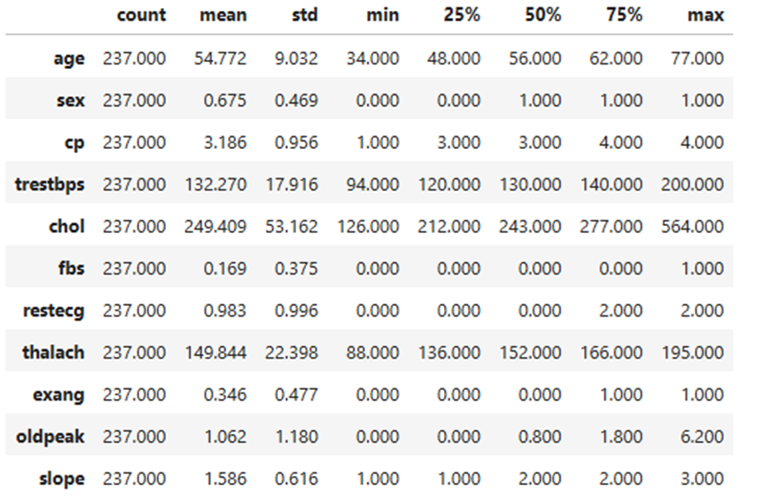
Univariate analysis of the Cleveland training set

The dataset reveals patterns about the participants and their health indicators. Most participants middle-aged, fall between 55 and 65 years old, with males having a majority within the dataset (see Table 1). When it comes to those experiencing chest pain, this had the highest severity (type 4). Both resting blood pressure and cholesterol levels show right-skewed distributions, indicating that while most values are moderate, some individuals have significantly higher levels. Only a small proportion of participants had elevated fasting blood sugar, suggesting that this issue is less common in the dataset. The resting electrocardiogram, the results appear to be normally distributed, showing a balanced spread of values.

The ‘exang’ is a variable that indicates the presence of an exercise-induced angina (1 for presence, 0 for absence), and is inferred from the low mean (see Table 1). The variable reveals that most participants do not experience angina during exercise and suggests that exercise-induced chest pain is less common in this dataset. However, the subset of individuals with a positive value for exang may represent a higher risk for underlying heart issues. Angina during exercise is often a significant indicator leading to coronary artery disease. (see Table 2) (see Table 3).

The distribution of values for the maximum heart rate feature has a strong left skew. Based on this left skew, we

 see most participants have a maximum heart rate above 140 beats per minute. The old peak feature, which measures changes in the ST segment of an ECG during exercise, indicates that most participants have values between 0 and 2, reflecting minimal ST depression and better heart health. However, there is a smaller group with higher values (up to 6).

The variable labeled ‘slope’, which describes the shape of the ST segment during peak exercise, shows that most participants have a flat slope (category 2). A smaller number have an upsloping slope (category 1), or a down sloping slope (category 3).

Relationships between distinct variables

A series of scatter points were created to understand the relationship between the distinct variable’s characteristics. The diagonals on the pair plot contain histograms depicting the distribution of specific features. The off-diagonal scatter plots show correlations between pairs of variables. For instance, age and cholesterol show a clear trend where greater cholesterol levels are related directly with older individuals.

The pair plot shows value distributions and feature relationships in the Cleveland training dataset. Age and maximum heart rate (thalach) exhibit a mild negative correlation, while Oldpeak (ST depression) and Slope display a stronger linear relationship, supporting their combination in feature engineering. Cholesterol (chol) and resting blood pressure (trestbps) have right-skewed distributions with noticeable outliers.

A correlation heatmap was utilized to identify and emphasize strong relationships among variables. Notable findings include a strong positive correlation between the slope of the ST segment and Oldpeak (r = 0.59), indicating a close association between these features. Age and maximum heart rate (thalach) show a moderate negative correlation (r = -0.35), suggesting that older individuals tend to have lower maximum heart rates. Additionally, chest pain type (cp) exhibits a moderate positive correlation with exercise-induced angina (exang, r = 0.36), highlighting a link between specific chest pain types and exercise-related symptoms. Mild correlations were also observed between sex and thalassemia (thal, r = 0.37), as well as age and the number of major vessels (ca, r = 0.37). Conversely, thalach displays weak negative correlations with several variables, including slope (r = -0.38) and Oldpeak (r = -0.36). These insights, highlighted in Figure 1, reveal key variable interactions that can inform the development of predictive models for heart disease.

Figure 1

Correlation amongst individual variables

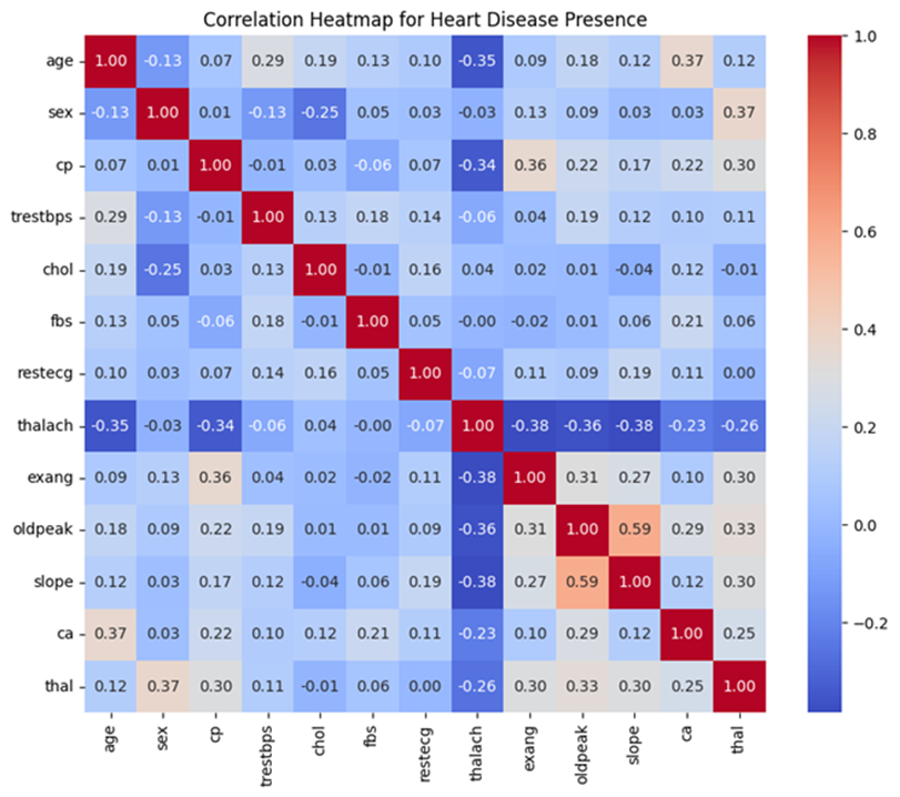
Distribution of heart disease presence in the training data.

            A bar chart was used to illustrate the distribution for binary classification of heart disease, distinguishing between presence (values 1–4) and absence (value 0).

 The distribution is slightly imbalanced, with more individuals in the “no heart disease” category compared to the “heart disease” category. In the training set, 128 patients did not have heart disease while there were 109 patients that indicated some level of presence for heart disease. This imbalance, while not extreme, could influence model performance. It is important to note that in a population-representative sample, most people are more likely to be free of heart disease than to have it.  

Analyzing individual variable association with heart disease presence.

            The analysis highlights different relationships between each feature and the presence of heart disease. A weak but statistically significant positive correlation was observed between age and heart disease, with older individuals modestly more likely to have heart disease (Point-Biserial Correlation Coefficient: 0.1990, p-value: 0.002085). Gender-based analysis revealed some notable patterns, with males more likely to have heart disease and females predominantly without it. This association was statistically significant (p-value: 3.26e-04). Similarly, higher chest pain types showed a strong relationship with heart disease presence. Particularly type 4 (asymptomatic chest pain), was more common among individuals with heart disease (Chi-Square test statistic: 65.29635, p-value: 4.33e-14). (see Table 2) (see Table 3)

Resting blood pressure was significantly higher among individuals with heart disease and exhibited greater variability (Point-Biserial Correlation Coefficient: 0.1632, p-value: 0.01188). Comparatively, cholesterol levels were slightly higher on average among those with heart disease, however, the relationship was not statistically significant (Point-Biserial Correlation Coefficient: 0.0661, p-value: 0.31068). Fasting blood sugar levels showed no meaningful association with heart disease. Most individuals in both groups had normal levels (Chi-Square test statistic: 0.00129, p-value: 0.9710).  The resting electrocardiogram results (restecg) demonstrated a strong association with abnormal results (restecg = 2), and was more common in individuals with heart disease. Normal results (restecg = 0) were prevalent among those without (Chi-Square test statistic: 35.63319, p-value: 2.38e-09). (see Table 2) (see Table 3).

Maximum heart rate (thalach) was inversely correlated with heart disease presence, with lower heart rates more common among individuals with heart disease (negative correlation coefficient, p-value < 0.05). Exercise-induced angina (exang) was noticeably more prevalent in those with heart disease (p-value: 2.38e-09). Oldpeak (ST depression) and slope (the slope of the ST segment during exercise) also exhibited a strong relationship with heart disease and with Oldpeak values (p-value < 0.05). Sharing their relationship with stress test outcomes and heart ischemia markers (see Table 2) (see Table 3).

In summary, the analysis underscores the importance of features such as Oldpeak, slope, chest pain type, and exercise-induced angina as strong indicators of heart disease. While expected trends like the link between age, vascular blockages, and declining cardiovascular efficiency were evident, weaker relationships for variables like cholesterol and fasting blood sugar highlight additional factors which were not associated with heart disease presence.

Table 2

Variable descriptives based on heart disease presence

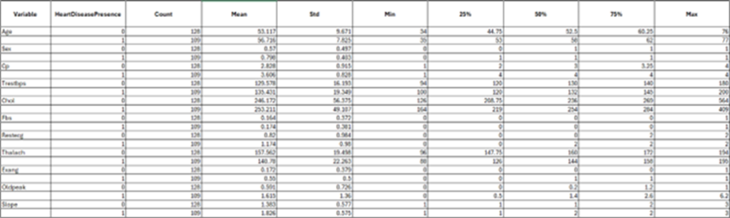
Table 3

Correlation Statistic between individual variables and heart disease presence

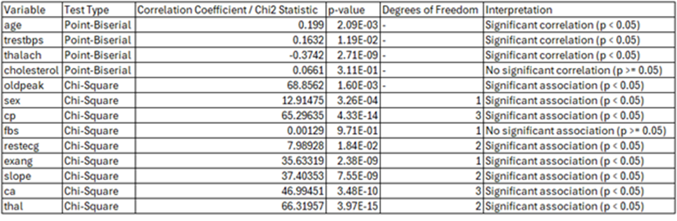
Coding environment

Google Colab, short for “Colaboratory,” is a cloud-based platform that allows users to write and execute Python code directly in their web browsers. Requiring no setup, it provides free access to GPUs for accelerated computation and facilitates easy sharing of projects. Google Colab’s computational resources and capabilities are leveraged throughout this project to write and execute code. Allowing a seamless workflow for analysis and modeling.

Coding language

            Python is a high-level and versatile programming language and is a central tool for this project. Python facilitates efficient code development for tasks such as data analysis, machine learning, and scientific computing (Python Software Foundation, 2024). Python has a robust standard library and a wide array of third-party packages, providing the necessary tools to handle complex data processing, build predictive models, and perform statistical analyses.

Python libraries

Several Python libraries that are essential for data manipulation, analysis, visualization, and machine learning are used within my research. NumPy serves as a fundamental package for numerical computations, offering support for arrays and matrices alongside a wide range of mathematical functions for handling large datasets. Complementing this is Pandas, which provides data structures similar to Data Frames that streamline the management and analysis of structured data. For visualization, Matplotlib and Seaborn are utilized. Matplotlib facilitates the creation of static visualizations, while Seaborn, built on Matplotlib, enhances statistical graphics through a high-level interface

For machine learning tasks, the notebook relies heavily on Scikit-learn and XGBoost. Scikit-learn is a versatile library that provides tools for preprocessing, model selection, and the implementation of machine learning algorithms, including classification, regression, clustering, and dimensionality reduction. XGBoost, known for its high efficiency and flexibility, is an optimized gradient boosting library designed for supervised learning tasks, particularly large-scale problems. Together, these libraries create a robust framework for data loading, preprocessing, visualization, and the implementation of advanced machine learning algorithms. By integrating these tools, the notebook demonstrates a comprehensive approach to solving binary classification problems, emphasizing both performance and interpretability.          

Splitting into training and testing sets

Before conducting model evaluation, it is essential to split data into training and testing sets. Splitting data into training and testing sets is crucial for building reliable machine learning models. The training set is used to teach the model by allowing it to learn patterns from the data, while the testing set evaluates the model’s performance on unseen data. This helps ensure that the model generalizes well and performs accurately on new, real-world data, reducing the risk of overfitting, where the model may perform well on training data but poorly on new data.

To effectively train and evaluate the binary classification model, the dataset was partitioned into training and testing subsets using the train_test_split function from the sklearn.model_selection module. The feature set (X) was created by removing the target column (num_binary)/ (Heart Disease Presence) from the dataset df_binary_col, while the target variable (y) was isolated as the column num_binary. This ensured that only relevant features were included in the model training process while preserving the target variable for prediction.

The data was split such that 80% of the samples were allocated to the training set and 20% to the testing set, specified by the test_size=0.2 parameter. To ensure reproducibility, a fixed random seed (random_state=42) was used, enabling consistent splitting of the dataset across different runs. Additionally, the stratify=y parameter was employed to maintain the proportional distribution of the binary target variable across both subsets. This stratification ensured that the training and testing sets were representative of the overall class distribution, reducing the risk of bias and enhancing the reliability of the model evaluation. This method of data splitting forms a robust foundation for training machine learning models and assessing their generalization capabilities.

To ensure robustness, multiple train-test splits were conducted for each experiment in order to maintain consistency for model performance. After the general train-test split, the test set (X_test) was further divided into male and female subsets. This additional split aimed to evaluate the model’s performance separately for each biological sex. The male and female subsets were used exclusively for testing, ensuring no overlap with the training data to maintain unbiased evaluations. This approach allowed for a detailed assessment of model generalizability for both men and women.

Exploratory data analysis (eda on x_train, Cleveland only)

            Exploratory Data Analysis (EDA) was conducted exclusively on the X_train subset of Cleveland’s dataset to understand its structure and guide subsequent transformations and modeling decisions while avoiding data leakage. This analysis included univariate analysis of each variable, how each variable relates to each other, as well as, examining variable distributions and their relationships with the target variable (heart disease presence), which provided insights into the underlying data characteristics. Correlation analysis was performed to detect multicollinearity and redundant features, ensuring that highly correlated variables were appropriately managed in later steps. Additionally, data visualization and transformation were applied to identify and address skewed data that could impact model performance.

To assess the relationship between individual features and heart disease presence, Chi-square tests were performed for categorical variables, such as chest pain type (cp) and sex, to determine significant associations. Continuous variables, including age and resting blood pressure (restbps), were evaluated using point-biserial correlation to assess their linear relationship with the binary target variable. Both tests provided critical insights into feature relevance and informed decisions about feature selection and weighting during the modeling process. The insights gained through EDA also guided transformation strategies, including the application of log transformations to normalize skewed variables like cholesterol (chol) and oldpeak. Notably, EDA was not performed for the VA Long Beach dataset, as this data was reserved exclusively for validation to maintain the integrity of the evaluation process.

Data cleaning: Cleveland

Although there were no NULL values in the dataset, six rows contained the value “?” to indicate missing data. Since this affected only a small number of records, all six rows were removed.

Data cleaning: VA Long Beach

The data cleaning process for the VA Long Beach dataset was significantly more intricate compared to cleaning the Cleveland dataset, reflecting the increased complexity of the data, regarding the level of missing values. This thorough process was essential to address the challenges of missing values, outliers, and inconsistencies, ensuring the dataset’s readiness for accurate binary classification modeling.

The first step involved removing columns with excessive missing values (ca and thal), as identified through visualizations. This step reduced noise while retaining the most informative features. For the remaining columns, a set of imputation strategies were implemented to handle missing values based on their data characteristics. Numerical columns with a normal distribution, such as restbps and thalach, were addressed using mean imputation, where missing values were replaced with the column’s mean. In contrast, median imputation was applied to skewed numerical columns, including chol and oldpeak, ensuring that the imputation process did not distort the data’s central tendency. For skewed categorical or binary columns (fbs, exang, and slope), mode imputation was employed, replacing missing values with the most frequently occurring category.

Outlier handling posed another challenge. Continuous numerical columns (restbps, chol, thalach, and oldpeak) were processed using the Interquartile Range (IQR) method. This approach identified outliers as values outside 1.5 times the IQR from the first and third quartiles. These outliers were clipped to the calculated bounds, effectively reducing their influence while preserving the overall data distribution.

Following imputation and outlier handling, any additional rows with missing values were removed. The corresponding target labels (y_train and y_test) were realigned to maintain consistency with the cleaned feature datasets. This ensured a seamless alignment of the feature-target pairs, critical for effective model training and evaluation.

To validate the cleaning process, the datasets were examined to confirm the absence of missing values, and descriptive statistics were reviewed to verify that outliers had been successfully addressed. These verification steps confirmed the data sets’ integrity, ensuring they were free of anomalies and inconsistencies.

Data transformation and feature engineering

            Three distinct data transformation/feature engineering experiments were applied to the Cleveland dataset to evaluate their impact on model performance. These experiments aimed to address issues such as skewness, scaling, and feature encoding to enhance the predictive power of the models. Based on performance evaluation metrics from the Cleveland dataset, the best-performing data transformation and feature engineering strategy was subsequently applied to the VA Long Beach dataset to ensure consistency and generalizability.

Transformation experiments on Cleveland dataset

Comparing logarithmic data transformation.

To extract meaningful results from our machine learning models, it is important to account for outlier values. An outlier indicates a value which is significantly different in value from the rest of the dataset. These values can negatively affect how well a machine learning model can generalize results, as they affect the performance and accuracy of a model (Mueller and Guido, 2016).  Outliers can be removed or accounted for using data transformation. Methods, such as logarithmic transformation, can reduce the impact of large outlier values. Alternatively, we can use square root transformation as well which is suitable for positively skewed data (Mueller and Guido, 2016).

For the following experiments, trestbps (resting blood pressure) and chol (cholesterol), and oldpeakwere transformed using a logarithmic scale because their distributions are right-skewed.

Side-by-side histograms were created to show the original and log-transformed distributions for resting blood pressure, cholesterol, and oldpeak (ST depression). The first histogram of the original data revealed a strong right skew for all three features. After log transformation, we observed a clear reduction in skewness. For resting blood pressure and cholesterol, the transformed data shows a significantly more symmetrical shape, indicating that the log transformation effectively normalized these distributions. For oldpeak, while the transformation reduces the skewness, the distribution remains slightly asymmetrical due to the heavy concentration of values near zero. These visual comparisons illustrate how log transformation reshapes the data, making it better suited for modeling and statistical analysis.

Comparing squared data transformation

Thalach (maximum heart rate achieved) has a left-skewed distribution. Therefore, a square transformation was applied to determine if this transformation better normalized the distribution. These visual comparisons highlight the impact of squared transformation on the data’s structure, making it clearer how the technique improves the suitability of these features for modeling and statistical analysis

In the first histogram with the original data, there is a slightly longer tail extending toward the lower values, indicating a right skewness. The outlying values seem to be patients with a low maximum heart rate. The histogram that represents the squared-transformed data amplified the range of values, particularly for higher maximum heart rates, while slightly smoothing the irregularities in the original data. This results in a slightly more normal distribution of values, although the overall symmetry of the distribution is preserved.

Transformation 1: logarithmic and square transformations

The first transformation experiment focused on reducing skewness and capturing non-linear relationships within the Cleveland dataset by applying two custom transformations: logarithmic and square transformations. These transformations were implemented using scikit-learn’s BaseEstimator and TransformerMixin, enabling integration into preprocessing pipelines. The “Log Transformer” applied a logarithmic transformation (log1p) to specific features, including resting blood pressure (trestbps) and cholesterol (chol), to reduce skewness and normalize their distributions. This adjustment aimed to stabilize variance and improve the compatibility of these features with machine learning algorithms. Similarly, the “Square Transformer” squared the values of maximum heart rate (thalach) to emphasize larger differences and capture potential non-linear relationships. These transformations tailored the preprocessing pipeline to the unique characteristics of the dataset. The integration of these custom transformers into the pipeline ensured seamless preprocessing and highlighted the importance of feature-specific transformations in enhancing data suitability for machine learning models.

Additionally, continuous features such as age, sex, chest pain, fasting blood sugar, resting electrocardiogram results, exercise induced angina, oldpeak, and slope are normalized using `StandardScaler` to ensure they have a mean of zero and a standard deviation of one. Categorical features, including ‘number of major vessels (ca)’, and ‘thalassemia (thal)’, are converted into binary format using OneHotEncoder. Any columns not explicitly specified for transformation are dropped, ensuring the preprocessing pipeline is both precise and adaptable to the dataset’s needs.

Transformation 2: logarithmic, square, and combined features

The second transformation experiment extended the preprocessing strategy by incorporating logarithmic and square transformations alongside the creation of a new combined feature. As in the first experiment, logarithmic transformations were applied to resting blood pressure (trestbps) and cholesterol (chol) to address skewness and stabilize variance. Similarly, maximum heart rate (thalach) was squared to emphasize its higher values and capture non-linear relationships. Additionally, a combined feature, oldpeak_slope_combined, was created by summing Oldpeak (ST depression induced by exercise) and Slope (the slope of the peak ST segment). These features were identified as having a strong correlation (0.59), suggesting a synergistic relationship that could enhance predictive power. The combined feature aimed to capture the interaction between Oldpeak and Slope, representing their joint contribution to heart disease prediction. After the combined feature was created, the original columns were dropped to streamline the dataset. The transformed data was standardized and processed alongside other features in the pipeline, with the goal of improving model predictive accuracy through enhanced feature engineering.

Transformation 3: logarithmic, square, combined features, and gender-based engineering

The third transformation experiment built upon the second by introducing gender-specific feature engineering to account for potential differences between male and female subgroups. As in the previous experiments, logarithmic transformations were applied to resting blood pressure (restbps) and cholesterol (chol), while maximum heart rate (thalach) was squared to capture non-linear relationships. The combined feature, oldpeak_slope_combined, was also created by summing Oldpeak and Slope to leverage their correlated relationship. In addition to these transformations, gender-based interactions were introduced to explore potential differences in feature relevance across genders. Interaction terms between gender and key features, such as cholesterol and resting blood pressure, were generated and integrated into the pipeline to evaluate their impact on model performance. By incorporating gender-aware feature engineering, this experiment aimed to enhance the model’s ability to predict heart disease while accounting for demographic-specific variations. The transformed data was processed within a standardized pipeline, ensuring compatibility and consistency across features.

Parameter tuning

            Three machine learning models—Random Forest Classifier, XGBoost Classifier, and an Ensemble Method combining the predictions from these two classifiers plus a logistic regression model—were used to evaluate the performance of each transformation strategy applied to the Cleveland dataset. For each model, a parameter grid search was conducted to optimize hyperparameters and enhance performance. This process involved systematically testing combinations of parameters, such as the number of estimators, maximum depth, learning rate, and feature split criteria, to identify the optimal configuration for each model. After parameter tuning, the models were trained and tested using multiple train-test splits to ensure robustness and mitigate the impact of variability. Performance metrics, including accuracy, precision, recall, and F1-score were calculated to comprehensively assess the predictive capabilities of each model under different transformations. The best-performing transformation was identified by selecting the strategy that achieved the highest average metrics across the evaluated models, ensuring both accuracy and reliability in subsequent applications.

To determine the most effective strategy for the Cleveland dataset, each experiment was evaluated using multiple performance metrics, including accuracy, precision, recall, F1-score, and AUC-ROC. These metrics provided an assessment of the models’ predictive capabilities. To ensure robustness and minimize the impact of variability in train-test splits, multiple splits were applied during the evaluation process.

Among the three transformation experiments, Transformation 2, which incorporated logarithmic transformations for resting blood pressure (trestbps) and cholesterol (chol), along with a squared transformation for maximum heart rate (thalach) and a combined feature (oldpeak_slope_combined), demonstrated the best overall performance. This strategy effectively balanced predictive accuracy with robustness across the evaluation metrics, making it the optimal choice for subsequent application to the VA.

Gender-based evaluation on Cleveland dataset

            Transformation 3 aimed to address gender differences identified during the exploratory analysis by introducing gender-specific feature engineering. This involved adding interaction terms between gender and key features, such as cholesterol and resting blood pressure, to capture sex-specific patterns and improve the model’s predictive performance for heart disease. The ensemble method, which combined the random forest classifier, XGBoost, and logistic regression, delivered the best results for this experiment.

On the testing data, the model demonstrated strong performance, achieving a mean accuracy of 0.85, an F1 score of 0.85, mean precision of 0.85, and recall of 0.85. Cross-validation revealed a significant drop in performance, with a mean accuracy of 0.77, mean precision of 0.79, mean recall of 0.77, and a mean F1 score of 0.76. These results indicate potential overfitting, as the model performed well on the testing data but struggled to generalize effectively across validation splits. Furthermore, the cross-validation results were worse than those achieved in previous experiments, Transformation 1 and Transformation 2.

Notably, Transformation 1 and Transformation 2 did not incorporate gender-specific parameter tuning, yet their cross-validation results outperformed Transformation 3. This suggests that while gender-aware parameter tuning improved performance on the test data, it introduced overfitting, reducing the model’s generalizability. As a result, the experiment with the best cross-validation performance was selected and further evaluated separately for men and women to ensure a more reliable assessment of its effectiveness.

To evaluate the performance of the best experiment (Transformation 2) and model across male and female subgroups, the Cleveland dataset’s test set was divided into male and female subsets based on the “sex” feature. Models trained using the best experiment (Transformation 2) were assessed separately for each gender. Key performance metrics, including accuracy, precision, recall, and F1-score were calculated for the male and female subsets to understand how the model performed across these demographic groups. This analysis provided valuable insights into potential gender-based discrepancies in model behavior, emphasizing the importance of ensuring fairness and robustness in predictive modeling across demographic subgroups.

Evaluation on VA Long Beach dataset

The best-performing strategy identified from the Cleveland dataset, Transformation 2, was applied to the VA Long Beach dataset to evaluate the regional generalizability of the trained model. This strategy included logarithmic transformations for features with skewed distributions, such as cholesterol (chol), resting blood pressure (trestbps), and Oldpeak, to stabilize variance and improve compatibility with the model. StandardScaler was then used to standardize continuous features, ensuring that all variables contributed equally during the model training and prediction process. Categorical variables were one-hot encoded, developed similarly as the Cleveland dataset to maintain consistency across the two regions. The goal of this approach was to investigate how a model trained exclusively on one region performs when applied to a different region with potentially varying feature distributions and population characteristics.

While a gender-based performance test was conducted for the Cleveland dataset, it could not be performed for the VA Long Beach dataset due to the limited representation of females in the dataset, with only six female observations. This small sample size precluded meaningful statistical analysis and comparison. Consequently, the gender-based analysis focused exclusively on the Cleveland dataset, where sufficient data for both male and female subgroups was available. By applying the same transformation strategy, the study aimed to make direct comparisons of overall model performance, assessing its robustness and ability to generalize across multiple cities in the U.S.

Application of the ascvd risk calculator to the Cleveland and VA Long Beach datasets

To further enhance the comparison of the predictive models, the ASCVD (Atherosclerotic Cardiovascular Disease) Risk Calculator was applied to both the Cleveland and VA Long Beach datasets. The ASCVD calculator, widely used in clinical settings, estimates the 10-year risk of cardiovascular disease based on key risk factors. The implementation was conducted using the Python package available in the GitHub repository https://github.com/brandones/ascvd/tree/master.

The ASCVD (Atherosclerotic Cardiovascular Disease) Risk Calculator was applied to both the Cleveland and VA Long Beach datasets to estimate the 10-year cardiovascular risk for individual patients. This ASCVD calculated risks using features such as age, sex, total cholesterol, HDL cholesterol, systolic blood pressure (SBP), blood pressure treatment status, diabetes status, and smoking status. Missing or unavailable data were addressed using proxies to ensure compatibility with the ASCVD model. HDL cholesterol was assigned a placeholder value of 50, and ethnicity was uniformly set to non-Black (isBlack = False) due to the absence of explicit data on this characteristic. Hypertension status was derived from SBP values, with readings of 130 or higher classified as hypertensive. Diabetes status was inferred from fasting blood sugar (fbs), with values over 120 converted into a boolean indicator (diabetic = True). Smoking status was approximated using exercise-induced angina (exang), treating the absence of angina as indicative of non-smoking status (False).

The use of proxies, such as placeholder HDL cholesterol values, inferred diabetes and smoking statuses, and uniform assumptions about ethnicity, underscores that the calculated risk scores are not pure ASCVD scores. These proxies, while necessary to accommodate missing or unavailable data, introduce approximations that deviate from the precise data required by the ASCVD model.

Introduction

The central focus of my capstone project is to explore the effectiveness of machine learning models in predicting heart disease and assess its ability to generalize across different cities and biological sexes. This research highlights the importance of building models that not only achieve high accuracy within a specific dataset or geographic location but are also reliable when applied to both men and women separately, as well as when applied to more than one city in the United States. Traditional cardiovascular risk scores, while reliable, exhibit limitations that impact its performance (Talha, Elkhoudri, and Hilali, 2024). Machine learning models have been shown, in previous research, to have better predictive accuracy than some cardiovascular risk scores (Cho, Kim, Kang, et al., 2021).

Studies have shown that traditional cardiovascular risk models frequently lack validation across diverse populations, leading to miscalculations and reduced sensitivity when applied to groups outside their original development context (Talha, Elkhoudri, and Hilali, 2024). This inability to generalize poses a challenge when providing accurate predictions for underrepresented groups, particularly women. Cardiovascular disease is the leading cause of death globally, responsible for 17.7 million deaths in 2015—a number expected to rise to over 23.6 million annually by 2030. Despite its prevalence, women tend to be undertreated, with their symptoms frequently misdiagnosed or dismissed as non-cardiac issues (Woodward, 2019).

This disparity underscores the urgent need to develop more inclusive and accurate predictive models. Women’s risk factors are often underestimated (Abdullah, Beckett, Wilson, et al., 2024). To address these challenges, my project uses machine learning models trained on data from both men and women, with performance tested separately for each gender. By addressing the limitations of traditional risk scores and accounting for differences in predictive accuracy for each gender, my project aims to more wholistically evaluate the accuracy and fairness of heart disease prediction. This is shown in my project when I compared the accuracy of the heart disease machine learning models to the ACSVD risk scores. This evaluation can help contribute to more equitable healthcare outcomes, by acting as an additional point of consideration.

Literature review

Heart disease prediction methods (risk models)

Multiple cardiovascular risk models have been made throughout the decades intended to accurately predict the risk of cardiovascular disease for the patients that used it. Understanding the strengths and limitations for each of these models is crucial for effective risk stratification and prevention strategies.

Over the past three decades, numerous risk prediction models have been developed to estimate an individual’s likelihood of developing cardiovascular disease (CVD). Among these, the multivariate risk prediction model from the Framingham Study has been particularly influential in estimating future CVD risk (Cui, 2009). Additional models have been created in the United States, such as the Reynolds Risk Score for women, derived from data collected in the Women’s Health Study. Other efforts include a “multi-marker” risk model that incorporates 10 genetic markers, including C-reactive protein and B-type natriuretic peptide (Cui, 2009).

In Europe, separate cardiovascular risk prediction models were developed due to the limited applicability of the Framingham risk scores to the general European population without recalibration (Cui, 2009). For example, the SCORE equation, endorsed by the Third Joint European Task Force on cardiovascular prevention, has been validated in Spain. In the UK, the QRISK algorithm was created using a population-based clinical research database. Germany contributed both a simple PROCAM score and a more complex neural network model, with the PROCAM score recently updated. Scotland developed the ASSIGN risk score, which includes family history of CVD, based on data from the Scottish Heart Health Extended Cohort. Italy introduced the CUORE equation tailored for populations with a low incidence of coronary events (Cui, 2009). These diverse models reflect efforts to address regional differences in CVD risk and provide tailored tools for prevention.

Major limitations of cardiovascular risk scores

A study conducted by Talha, Elkhoudri, and Hilali, in 2024, summarized the best-known limitations of current cardiovascular risk models. Critical analysis revealed numerous limitations that impact performance. Each calculator demonstrates distinct advantages for one population while potentially encountering limitations with another. Some scores lack validation from external cohorts, while others seem to miscalculate risk when applied to populations outside of its origin, limiting its sensitivity, and being unable to explain all cardiac events (Talha, Elkhoudri, and Hilali, 2024).

Numerous cardiovascular risk assessment tools have been developed from large population studies, but only a few have undergone essential external validation. The most common models, American and European scores, have distinct characteristics and limitations. Understanding these limitations is crucial for improving the effectiveness of these tools (Talha, Elkhoudri, and Hilali, 2024).

Comparisons of established risk prediction models for cardiovascular disease

A study, reviewing 74 previous research articles, aimed to evaluate and compare established cardiovascular risk prediction models to assess their performance. Investigators evaluated the performance of two or more risk prediction models in the same populations. The study extracted information on design, assessed models, and outcomes, examining their performance in terms of discrimination, calibration, and reclassification, while also considering biases favoring newer or author-developed models (Siontis, Tzoulaki, Siontis, et al., 2012).

The review included 74 articles, covering 56 pairwise comparisons of eight models, such as two variants of the Framingham risk score, ASSIGN score, SCORE, PROCAM score, QRISK1 and QRISK2 algorithms, and the Reynolds risk score. Only 10 of the 56 comparisons showed more than a 5% relative difference in predictive performance based on the area under the receiver operating characteristic curve (AUC). This means that most models had similar discriminatory abilities, as most comparisons did not exceed the 5% threshold. This suggests that these risk prediction models perform comparably in distinguishing between individuals at high and low risk of cardiovascular events. The use of other statistical measures like discrimination, calibration, and reclassification was inconsistent (Siontis, Tzoulaki, Siontis, et al., 2012). Outcome selection bias was evident in 32 comparisons, where 78% of the time, the model originally developed using the selected outcome performed better. Additionally, authors tended to report better AUCs for models they developed, highlighting potential optimism bias (Siontis, Tzoulaki, Siontis, et al., 2012).

The conclusions suggest that while multiple cardiovascular risk prediction models exist, their comparisons would benefit from standardized reporting and consistent statistical evaluation. The reporting/evaluation of these risk models appear to be impacted by outcome selection and optimism biases, emphasizing the need for more rigorous and unbiased comparisons (Siontis, Tzoulaki, Siontis, et al., 2012).

Gender bias in assessing cardiovascular disease

Cardiovascular disease (CVD) rates are higher in males, which has led to it being seen as primarily a men’s issue. However, CVD is the leading cause of death and a major cause of disability for women globally. Women are often under-recognized and undertreated for CVD compared to men, and their symptoms can differ, leading to worse outcomes. Female patients treated by male cardiologists fare worse than male patients, while no such difference exists for female cardiologists. Clinical trials often focus on men, despite some drugs having different effects in women. Risk factors like diabetes and smoking increase CVD risk more in women, and factors related to pregnancy and reproductive health add to their vulnerability. Women’s health research is often focused on mother and child health and breast cancer, neglecting CVD and other non-communicable diseases. There is a need to broaden the definition of women’s health to include the entire lifecycle and emphasize CVD, with sex-specific research analyses becoming standard (Abdullah, Beckett, Wilson, et al., 2024).

Additionally, a study reviewed the evidence on gender bias in CVD diagnosis, prevention, and treatment. Following PRISMA guidelines, several databases from 19 studies were searched and analyzed. The findings showed that CVD is less reported in women, who often have milder symptoms or are misdiagnosed with gastrointestinal or anxiety issues. As a result, women’s risk factors are often overlooked, especially by male doctors. Women are given fewer diagnostic tests and are less likely to be referred to cardiologists or hospitalized. Even when hospitalized, women receive fewer coronary interventions and are prescribed fewer cardiovascular medications, except for antihypertensive and anti-anginal drugs. Women also tend to perceive themselves at lower risk for CVD than men. This review highlights that women receive fewer diagnostic tests and treatments for CVD, which affects their health outcomes, likely due to a lack of awareness about gender differences in CVD symptoms (Abdullah, Beckett, Wilson, et al., 2024).

Most of this research is based on a gender binary frame, which assumes the existence of only two distinct and opposite genders—male and female—often neglecting the experiences of non-binary and gender-diverse individuals. This binary approach reinforces systemic gaps in understanding the intersection of gender and health outcomes, as it fails to account for how non-binary individuals experience, report, and are treated for CVD. The focus on a binary framework not only limits the inclusivity of cardiovascular research but also perpetuates disparities by oversimplifying the complex interplay of biological sex and gender identity. Expanding research to include non-binary and gender-diverse populations is crucial to developing a more comprehensive understanding of cardiovascular health and ensuring equitable healthcare practices for all individuals.

Pre-existing machine learning methods for predicting cardiovascular disease

Using machine learning methods to predict cardiovascular disease has been an ongoing point of research in the last decade. The following study focused on improving risk prediction using machine learning on healthcare data from 222,998 Korean adults aged 40-79 without prior cardiovascular disease or lipid-lowering therapy. Traditional risk models showed moderate to good performance (C-statistics 0.70–0.80), with the pooled cohort equation (PCE) achieving a C-statistic of 0.738 (Cho, Kim, Kang, et al., 2021). Among various machine learning models tested, the neural network model performed best, with a C-statistic of 0.751, which was higher than PCE. It also showed better agreement between predicted and actual outcomes. Improvements were noted compared to other models like the Framingham risk score, systematic coronary risk evaluation, and QRISK3 (Cho, Kim, Kang, et al., 2021). The study concluded that machine learning algorithms could enhance cardiovascular risk prediction beyond existing models, making them valuable tools for risk assessment and clinical decision-making in healthy Korean adults (Cho, Kim, Kang, et al., 2021).

Additionally, in a study by Stephen F. Weng and colleagues, machine learning was assessed for improving cardiovascular risk prediction using data from 378,256 UK patients. Four algorithms (random forest, logistic regression, gradient boosting, neural networks) were compared to the American College of Cardiology guidelines for evaluating CVD risk. The best-performing algorithm, neural networks, had an AUC of 0.764, improving prediction accuracy by 3.6% over the established method. This approach identified more patients who could benefit from preventive treatment and reduced unnecessary interventions (Weng, Reps, Kai, et al., 2017).

Gender-based approach for diagnosing coronary heart disease

            In 2019, Hogo published an article titled “A proposed gender‑based approach for diagnosis of coronary artery disease.” In this research article, two separate and individual models were trained and evaluated for each gender to determine whether the patient’s gender affects the structure and performance of a diagnosis model for coronary artery disease. The male diagnosis model achieved an accuracy of 95%, with a sensitivity of 96% and a specificity of 100%, while the female diagnosis model performed slightly better, with an accuracy of 96%, a sensitivity of 97%, and a specificity of 96%. The high-performance results overall highlight the success of the proposed gender-based approach for diagnosing coronary artery disease. The dataset used for this project is from the UCI Machine Learning Repository; specifically, the “Heart Disease Database” and the “Z-Alizadeh Sani Dataset,” which comprises records for 270 patients, each with 75 attributes (Hogo, 2020).

Supervised machine learning

My project uses multiple supervised machine learning algorithms on a clinical dataset to predict the presence of cardiovascular disease in patients. Supervised learning is a type of machine learning where the algorithm is trained on labeled data to make predictions or decisions (Mueller and Guido, 2016). It learns to map input data to the correct output. For this project, I conducted a classification task to predict whether a patient has heart disease. Classification is one of the two primary types of supervised learning problems in machine learning (Mueller and Guido, 2016). Specifically, this project focused on binary classification, which involves distinguishing between two distinct classes (Mueller and Guido, 2016). The results of different machine learning models, such as a Random Forest Classifier, and XGB Classifier, were compared with cross-validation, which was used to ensure the reliability of the performance estimates.

A random forest classifier is a type of ensemble method, that combines multiple decision trees to create a more powerful model. Decision trees are a type of diagram/logic that is widely used for classification tasks. Each decision tree is based off a hierarchy of “if/else” questions, leading to a decision tree. In a random forest model, each decision tree is slightly different from the others. The concept behind random forests is that while each individual tree can provide reasonably accurate predictions, it is prone to overfitting specific portions of the data. One decision tree might be overfit in one way, and another might be overfit in another. By averaging their results, one can retain the predictive power of decision trees while reducing overfitting. Random forests incorporate two levels of randomness: first, by selecting a random subset of data points to construct each tree, and second, by randomly selecting a subset of features to evaluate at each split (Mueller and Guido, 2016).

XGBoost, which stands for “Extreme Gradient Boosting”, is a highly efficient and scalable library for gradient boosting, specifically designed to optimize the training process of machine learning models. The XGBoost classifier is a gradient boost regression tree, which is another ensemble method that combines multiple decision trees to create a more powerful model. Unlike the random forest method, gradient boosting constructs trees sequentially, with each tree aiming to address the errors made by the preceding one (Mueller and Guido, 2016). The gradient boos trees are typically shallow, with a maximum depth of 1 to 5. These types of models would be considered “weak learners”, as they only capture a small portion of the data’s complexity. The main idea is to combine many of these models. Each tree can only provide good predictions on part of the data, and so more and more trees are added iteratively to improve performance (Mueller and Guido, 2016).  

Gradient boosting models are generally more sensitive to parameter settings compared to random forest classifiers. This increased sensitivity means that the performance of gradient boosting can vary significantly depending on how parameters are tuned. However, when parameters are properly optimized, gradient boosting has the potential to achieve higher accuracy than random forests (Mueller and Guido, 2016).

Machine learning models were evaluated by calculating the F1-score, recall score, accuracy score, and precision score. The precision score measures how many predicted positive instances were correct. Accuracy measures the overall correctness of the model. The recall score focuses on how well a model evaluated negative prediction. For this dataset, a model is considered to have a negative prediction if a patient is not diagnosed at all with cardiovascular disease. The F1-score combines precision and recall into a single number, balancing the trade-offs. It is the average of precision and recall, with a greater emphasis on the smaller value. The score goes from 0 to 100%, with higher values indicating better performance. It is particularly useful for imbalanced datasets because it considers both false positives and false negatives (Mueller and Guido, 2016).

For this capstone project, I investigated how well machine learning models can predict heart disease, while also studying how the patient’s gender affects these predictions, as well as determining how well the same model performs across different regions. This project utilizes two clinical datasets from the publicly accessible UCI Machine Learning Repository under the collection “Heart Disease.” This repository is composed of data from patients across four distinct locations, capturing varying levels of heart disease severity. These datasets are part of a collection of databases, open to the public, and can be used by anyone looking to conduct empirical analysis.

For this study, I specifically focused on two of the four datasets available: the “processed. cleveland.data,” which contains patient records from Cleveland, and the “processed.va.data,” which includes data from the Veterans Administration in Long Beach. These datasets provided my foundation for analyzing heart disease risk factors and evaluating predictive models. This project evaluated the predictive accuracy of machine learning algorithms and compared its performance to traditional cardiovascular risk scores, such as the American College of Cardiology’s Atherosclerotic Cardiovascular Disease (ASCVD). Furthermore, I investigated the expectations of a machine learning models’ ability to surpass the predictive accuracy of established ASCVD risk scoring. I also examined whether significant differences arose when evaluating the model’s predictive performance for men and women, as well as when applying the same model to datasets from two different cities. This dual focus aims to uncover both gender-specific variations and location-based disparities in model effectiveness.

For my research, I applied the following machine learning algorithms: Random Forest, XGBoost, and an ensemble method combining them. These algorithms were applied to heart disease prediction datasets, using tailored preprocessing and feature engineering techniques.

Three distinct experiments were conducted, each labeled Transformation 1, Transformation 2, and Transformation 3. Transformation 1 normalized skewed data and applied squared transformations to capture non-linear relationships. Transformation 2 introduced engineered features such as the combination of ST depression (Oldpeak) with the slope of the ST segment. Transformation 3 incorporated a custom feature to account for gender differences. Exploratory analysis revealed that chest pain type, ST depression (Oldpeak), and exercise-induced angina were key predictors, while cholesterol and fasting blood sugar contributed little predictive value. The best experiment combined multiple elements from all these transformations and significantly improved the model’s performance and predictive accuracy.

The performance of the ASCVD risk score was also evaluated on both datasets to act as a benchmark against the machine learning models. For the Cleveland dataset, the ASCVD score achieved an accuracy of 69.64%, with a precision of 63.58%, recall of 79.14%, and an F1 score of 70.51%. Notably, the model performed better for females than males, with higher recall (88.89% vs. 77.19%) but lower precision (48.88% vs. 68.75%). This variability highlighted challenges in achieving consistent results for both men and women. On the VA Long Beach dataset, the ASCVD score achieved a higher accuracy of 76.82%, precision of 78.95%, and recall of 93.75%, yielding an F1 score of 85.71%. Due to an insufficient number of females in the VA Long Beach dataset, a sex-specific analysis was not feasible.

The Random Forest model utilizing Transformation 2 demonstrated the best overall predictive accuracy and better predictive accuracy compared to the ASCVD score, achieving 83.33% accuracy for the Cleveland dataset and 82.5% for the Long Beach dataset. However, gender-based disparities emerged in the model’s performance. The Random Forest Model performed better overall for the female subgroup in the Cleveland dataset, exhibiting a higher overall precision and recall, meaning that the model was better at making a correct prediction. However, the model exhibited a poor recall of 67% amongst patients with heart disease. This indicated that the model was not good at correctly predicting patients with heart disease. In contrast, the model had much more balanced predictive accuracy when evaluating the male subgroup.

The Transformation 2 experiment utilizing the Random Forest model performed well overall but demonstrated additional biases when evaluated on the Long Beach dataset. For example, in the Cleveland dataset, which had a relatively balanced distribution of heart disease and non-heart disease cases, the model was able to accurately identify both classes. However, in the VA Long Beach dataset, where heart disease cases were more prevalent, the model demonstrated a poor recall for the minority class in the dataset (“patients without heart disease”) while showing high precision and recall for the majority class (“heart disease”). This tendency resulted in a recall of 97% for heart disease cases, indicating the model was highly effective at identifying individuals with heart disease. The precision for heart disease was 83%, meaning 17% of those classified as having heart disease were false positives.

For non-heart disease cases, the model’s recall was only 40%, highlighting its inability to correctly identify most individuals without heart disease. This trade-off—favoring high recall for the majority class at the expense of accurately identifying minority class cases—illustrates the challenge of generalizing performance across datasets which include patients from different regions. The class imbalance only further reduces the ability to generalize these results.

Findings suggest that while my machine learning models hold promise for improving heart disease prediction, the gender imbalances and regional variations in these datasets limit the general utility of these findings. Due to the class imbalance, future research that utilizes these datasets should explore multilabel classification for varying disease severities and address sampling biases that arise from an overall low representation of women in these datasets. This will enhance both fairness and the model’s application across all populations.