Data

The UCI Machine Learning Repository is a comprehensive resource that provides databases, domain theories, and data generators widely utilized by the machine learning community for evaluating models. For the this project, I utilized the database titled “Heart Disease” available in the UCI machine Learning Repository. The “Heart Disease” database from the UCI Machine Learning Repository is a resource that can be used for evaluating models that classify cardiovascular disease. The database includes four distinct datasets, each comprised of anonymized patient records with various social and biological indicators—such as age, exercise-induced angina, and systolic blood pressure—alongside a target column that specifies whether the patient has heart disease and, if so, its severity.

There are four datasets available from four different regions: Cleveland, Hungary, Switzerland, and the VA Long Beach. There are 76 attributes, but all published experiments refer to using a subset of 14 of them. The “goal” field refers to the presence of heart disease in the patient.  It is integer valued from 0 (no presence) to 4. Most experiments have concentrated on simply attempting to distinguish presence (values 1,2,3,4) from absence (value 0) (Janosi, Steinbrunn, Pfisterer, et al., 1988).  That is what I did for this project. The datasets donated by UC Irvine consists of 76 attributes. However, the processed datasets that I used consisted of a subset of 13 of them. For the purposes of this project, I used the Cleveland dataset, as well as the VA Long Beach Dataset.

The processed Cleveland dataset includes 303 patient records, eachwith varying levels of heart disease severity. An additional dataset, consisting of patients from the United States was contributed to the database by the Veterans Administration of Long Beach, California. The VA Long Beach Healthcare System, formerly known as Naval Hospital Long Beach, encompasses a network of Veterans Administration facilities in Long Beach and nearby cities. This data set includes 200 patient records, most of whom have some degree of heart disease, and features the same 14 columns as the Cleveland dataset.

In both datasets, the presence of heart disease is indicated by values ranging from 1 to 4, corresponding to increasing severity, while a value of 0 represents the absence of the condition. Consistent with prior research on the Cleveland dataset, this study concentrates on distinguishing between the presence (values 1–4) and absence (value 0) of heart disease. The primary focus of my project was on analyzing binary classification.

This dataset provides clinical and demographic information about patients, focusing on attributes associated with heart disease risk. Key variables include age (in years) and sex (0 for female, 1 for male), along with cp (chest pain severity) categorized on a scale of 0 to 4. Diagnostic measurements include restbps (resting blood pressure in mmHg), chol. (serum cholesterol level in mg/dL), and fbs (fasting blood sugar), a binary variable indicating whether fasting blood sugar exceeds 120 mg/dL. Additionally, the dataset captures restecg (resting electrocardiographic results) with categories ranging from normal results to indications of left ventricular hypertrophy, and Thalach, which measures the maximum heart rate achieved.

Other features assess cardiovascular responses to stress, such as exang (exercise-induced angina, binary), oldpeak (ST segment depression on ECG during exercise), and slope, describing the pattern of the ST segment during peak exercise (upsloping, flat, or down sloping). The ca variable indicates the number of major vessels (0–3) visualized through fluoroscopy, and thal (a thalassemia-related variable indicating heart stress test results) which is also associated with increased heart disease severity. As a side note, this thalassemia related variable seems to become more pronounced as age increases. Each patient’s thallium stress test results were categorized as normal, fixed defect, or reversible defect. The target variable, num, ranges from 0 to 4, representing the presence and severity of heart disease. This dataset is comprehensive, combining demographic and clinical variables, making it suitable for exploring the factors influencing heart disease outcomes. To ensure privacy, patient names and social security numbers were removed from the database and replaced with de-identified data.

Exploratory data analysis results

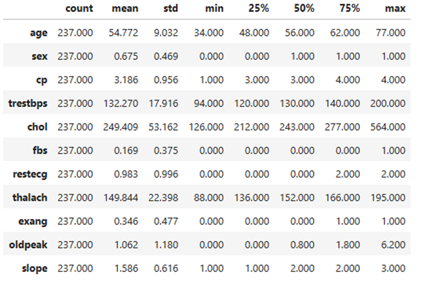
Basic descriptives of the Cleveland training set

            The training set for the Cleveland dataset provides insights into the demographic and clinical characteristics of individuals included in the study. The average age of participants is approximately 54.77 years, with ages ranging from 34 to 77 years and an interquartile range (IQR) of 48 to 62 years. The dataset has a higher proportion of males, with the mean value for sex coded as 0.675 (1 for males and 0 for females). For chest pain type (cp), the average value is 3.186, with a range of 1 to 4, reflecting a balanced range of values for classifications of chest pain. Resting blood pressure (trestbps) has a mean of 132.27 mmHg, ranging from 94 to 200 mmHg, with an IQR of 120 to 140 mmHg. The mean cholesterol level (chol) is 249.41 mg/dL, spanning from 126 to 564 mg/dL, and an IQR of 212 to 277 mg/dL.

Fasting blood sugar (fbs) shows a mean of 0.169, indicating a low prevalence of elevated fasting blood sugar (coded as 1 for high and 0 for normal). Maximum heart rate achieved (thalach) averages 149.84 bpm, with a range of 88 to 195 bpm and an IQR of 136 to 166 bpm. Exercise-induced angina (exang) is less frequent, with a mean of 0.346 (coded as 1 for yes and 0 for no). The mean ST depression induced by exercise (oldpeak) is 1.062, ranging from 0 to 6.2, with an IQR of 0 to 1.8. Finally, the slope of the peak exercise ST segment (slope) has an average value of 1.586, with values ranging from 1 to 3, representing a balanced range of values for slope categories. These descriptive statistics highlight key trends and distributions in the dataset.    

Table 1

Basic Descriptives of the Cleveland training data

Univariate analysis of the Cleveland training set

The dataset reveals patterns about the participants and their health indicators. Most participants middle-aged, fall between 55 and 65 years old, with males having a majority within the dataset (see Table 1). When it comes to those experiencing chest pain, this had the highest severity (type 4). Both resting blood pressure and cholesterol levels show right-skewed distributions, indicating that while most values are moderate, some individuals have significantly higher levels. Only a small proportion of participants had elevated fasting blood sugar, suggesting that this issue is less common in the dataset. The resting electrocardiogram, the results appear to be normally distributed, showing a balanced spread of values.

The ‘exang’ is a variable that indicates the presence of an exercise-induced angina (1 for presence, 0 for absence), and is inferred from the low mean (see Table 1). The variable reveals that most participants do not experience angina during exercise and suggests that exercise-induced chest pain is less common in this dataset. However, the subset of individuals with a positive value for exang may represent a higher risk for underlying heart issues. Angina during exercise is often a significant indicator leading to coronary artery disease. (see Table 2) (see Table 3).

The distribution of values for the maximum heart rate feature has a strong left skew. Based on this left skew, we

 see most participants have a maximum heart rate above 140 beats per minute. The old peak feature, which measures changes in the ST segment of an ECG during exercise, indicates that most participants have values between 0 and 2, reflecting minimal ST depression and better heart health. However, there is a smaller group with higher values (up to 6).

The variable labeled ‘slope’, which describes the shape of the ST segment during peak exercise, shows that most participants have a flat slope (category 2). A smaller number have an upsloping slope (category 1), or a down sloping slope (category 3).

Relationships between distinct variables

A series of scatter points were created to understand the relationship between the distinct variable’s characteristics. The diagonals on the pair plot contain histograms depicting the distribution of specific features. The off-diagonal scatter plots show correlations between pairs of variables. For instance, age and cholesterol show a clear trend where greater cholesterol levels are related directly with older individuals.

The pair plot shows value distributions and feature relationships in the Cleveland training dataset. Age and maximum heart rate (thalach) exhibit a mild negative correlation, while Oldpeak (ST depression) and Slope display a stronger linear relationship, supporting their combination in feature engineering. Cholesterol (chol) and resting blood pressure (trestbps) have right-skewed distributions with noticeable outliers.

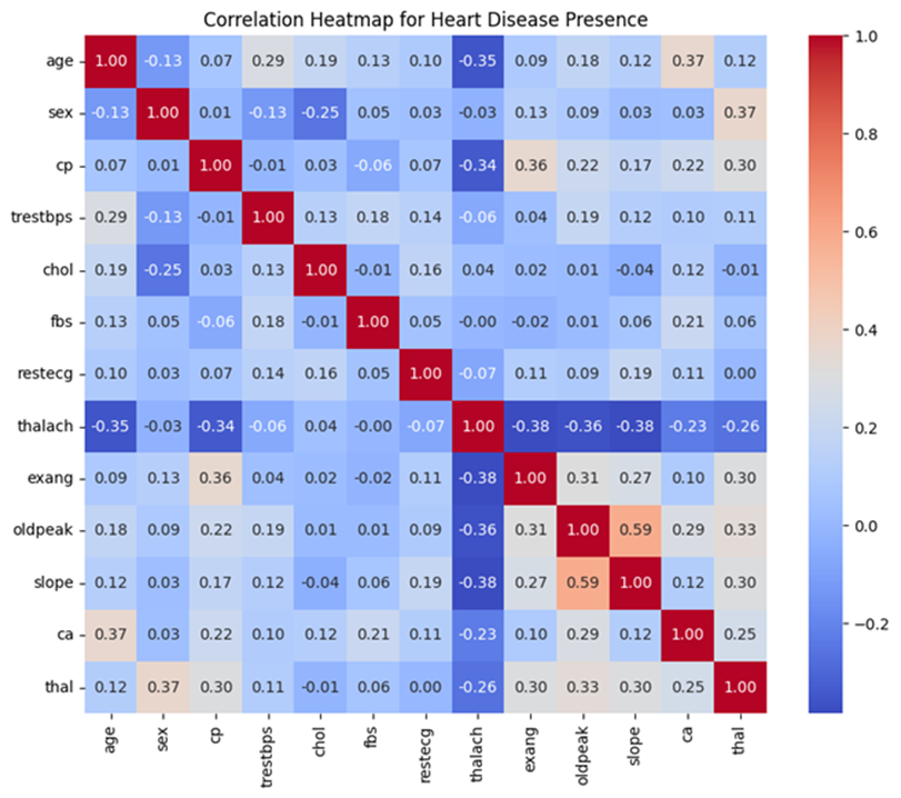
A correlation heatmap was utilized to identify and emphasize strong relationships among variables. Notable findings include a strong positive correlation between the slope of the ST segment and Oldpeak (r = 0.59), indicating a close association between these features. Age and maximum heart rate (thalach) show a moderate negative correlation (r = -0.35), suggesting that older individuals tend to have lower maximum heart rates. Additionally, chest pain type (cp) exhibits a moderate positive correlation with exercise-induced angina (exang, r = 0.36), highlighting a link between specific chest pain types and exercise-related symptoms. Mild correlations were also observed between sex and thalassemia (thal, r = 0.37), as well as age and the number of major vessels (ca, r = 0.37). Conversely, thalach displays weak negative correlations with several variables, including slope (r = -0.38) and Oldpeak (r = -0.36). These insights, highlighted in Figure 1, reveal key variable interactions that can inform the development of predictive models for heart disease.

Figure 1

Correlation amongst individual variables

Distribution of heart disease presence in the training data.

            A bar chart was used to illustrate the distribution for binary classification of heart disease, distinguishing between presence (values 1–4) and absence (value 0).

 The distribution is slightly imbalanced, with more individuals in the “no heart disease” category compared to the “heart disease” category. In the training set, 128 patients did not have heart disease while there were 109 patients that indicated some level of presence for heart disease. This imbalance, while not extreme, could influence model performance. It is important to note that in a population-representative sample, most people are more likely to be free of heart disease than to have it.  

Analyzing individual variable association with heart disease presence.

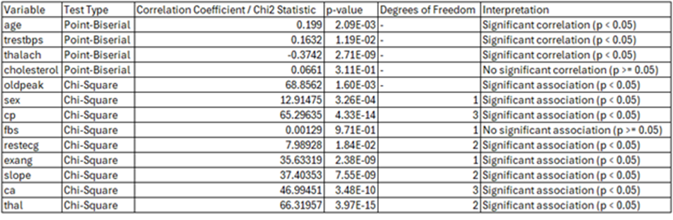
            The analysis highlights different relationships between each feature and the presence of heart disease. A weak but statistically significant positive correlation was observed between age and heart disease, with older individuals modestly more likely to have heart disease (Point-Biserial Correlation Coefficient: 0.1990, p-value: 0.002085). Gender-based analysis revealed some notable patterns, with males more likely to have heart disease and females predominantly without it. This association was statistically significant (p-value: 3.26e-04). Similarly, higher chest pain types showed a strong relationship with heart disease presence. Particularly type 4 (asymptomatic chest pain), was more common among individuals with heart disease (Chi-Square test statistic: 65.29635, p-value: 4.33e-14). (see Table 2) (see Table 3)

Resting blood pressure was significantly higher among individuals with heart disease and exhibited greater variability (Point-Biserial Correlation Coefficient: 0.1632, p-value: 0.01188). Comparatively, cholesterol levels were slightly higher on average among those with heart disease, however, the relationship was not statistically significant (Point-Biserial Correlation Coefficient: 0.0661, p-value: 0.31068). Fasting blood sugar levels showed no meaningful association with heart disease. Most individuals in both groups had normal levels (Chi-Square test statistic: 0.00129, p-value: 0.9710).  The resting electrocardiogram results (restecg) demonstrated a strong association with abnormal results (restecg = 2), and was more common in individuals with heart disease. Normal results (restecg = 0) were prevalent among those without (Chi-Square test statistic: 35.63319, p-value: 2.38e-09). (see Table 2) (see Table 3).

Maximum heart rate (thalach) was inversely correlated with heart disease presence, with lower heart rates more common among individuals with heart disease (negative correlation coefficient, p-value < 0.05). Exercise-induced angina (exang) was noticeably more prevalent in those with heart disease (p-value: 2.38e-09). Oldpeak (ST depression) and slope (the slope of the ST segment during exercise) also exhibited a strong relationship with heart disease and with Oldpeak values (p-value < 0.05). Sharing their relationship with stress test outcomes and heart ischemia markers (see Table 2) (see Table 3).

In summary, the analysis underscores the importance of features such as Oldpeak, slope, chest pain type, and exercise-induced angina as strong indicators of heart disease. While expected trends like the link between age, vascular blockages, and declining cardiovascular efficiency were evident, weaker relationships for variables like cholesterol and fasting blood sugar highlight additional factors which were not associated with heart disease presence.

Table 2

Variable descriptives based on heart disease presence

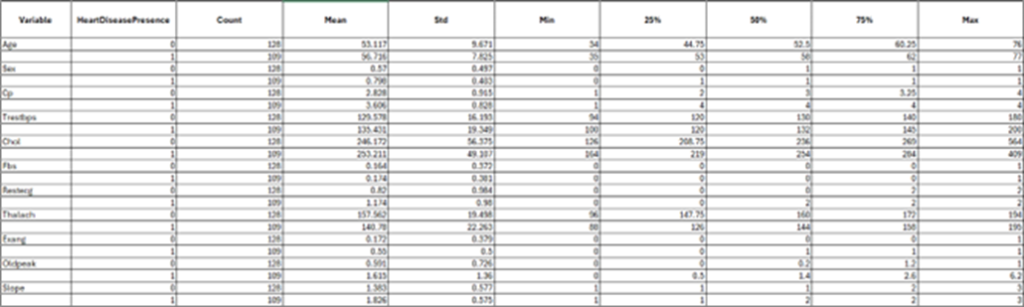
Table 3

Correlation Statistic between individual variables and heart disease presence

Coding environment

Google Colab, short for “Colaboratory,” is a cloud-based platform that allows users to write and execute Python code directly in their web browsers. Requiring no setup, it provides free access to GPUs for accelerated computation and facilitates easy sharing of projects. Google Colab’s computational resources and capabilities are leveraged throughout this project to write and execute code. Allowing a seamless workflow for analysis and modeling.

Coding language

            Python is a high-level and versatile programming language and is a central tool for this project. Python facilitates efficient code development for tasks such as data analysis, machine learning, and scientific computing (Python Software Foundation, 2024). Python has a robust standard library and a wide array of third-party packages, providing the necessary tools to handle complex data processing, build predictive models, and perform statistical analyses.

Python libraries

Several Python libraries that are essential for data manipulation, analysis, visualization, and machine learning are used within my research. NumPy serves as a fundamental package for numerical computations, offering support for arrays and matrices alongside a wide range of mathematical functions for handling large datasets. Complementing this is Pandas, which provides data structures similar to Data Frames that streamline the management and analysis of structured data. For visualization, Matplotlib and Seaborn are utilized. Matplotlib facilitates the creation of static visualizations, while Seaborn, built on Matplotlib, enhances statistical graphics through a high-level interface

For machine learning tasks, the notebook relies heavily on Scikit-learn and XGBoost. Scikit-learn is a versatile library that provides tools for preprocessing, model selection, and the implementation of machine learning algorithms, including classification, regression, clustering, and dimensionality reduction. XGBoost, known for its high efficiency and flexibility, is an optimized gradient boosting library designed for supervised learning tasks, particularly large-scale problems. Together, these libraries create a robust framework for data loading, preprocessing, visualization, and the implementation of advanced machine learning algorithms. By integrating these tools, the notebook demonstrates a comprehensive approach to solving binary classification problems, emphasizing both performance and interpretability.          

Splitting into training and testing sets

Before conducting model evaluation, it is essential to split data into training and testing sets. Splitting data into training and testing sets is crucial for building reliable machine learning models. The training set is used to teach the model by allowing it to learn patterns from the data, while the testing set evaluates the model’s performance on unseen data. This helps ensure that the model generalizes well and performs accurately on new, real-world data, reducing the risk of overfitting, where the model may perform well on training data but poorly on new data.

To effectively train and evaluate the binary classification model, the dataset was partitioned into training and testing subsets using the train_test_split function from the sklearn.model_selection module. The feature set (X) was created by removing the target column (num_binary)/ (Heart Disease Presence) from the dataset df_binary_col, while the target variable (y) was isolated as the column num_binary. This ensured that only relevant features were included in the model training process while preserving the target variable for prediction.

The data was split such that 80% of the samples were allocated to the training set and 20% to the testing set, specified by the test_size=0.2 parameter. To ensure reproducibility, a fixed random seed (random_state=42) was used, enabling consistent splitting of the dataset across different runs. Additionally, the stratify=y parameter was employed to maintain the proportional distribution of the binary target variable across both subsets. This stratification ensured that the training and testing sets were representative of the overall class distribution, reducing the risk of bias and enhancing the reliability of the model evaluation. This method of data splitting forms a robust foundation for training machine learning models and assessing their generalization capabilities.

To ensure robustness, multiple train-test splits were conducted for each experiment in order to maintain consistency for model performance. After the general train-test split, the test set (X_test) was further divided into male and female subsets. This additional split aimed to evaluate the model’s performance separately for each biological sex. The male and female subsets were used exclusively for testing, ensuring no overlap with the training data to maintain unbiased evaluations. This approach allowed for a detailed assessment of model generalizability for both men and women.

Exploratory data analysis (eda on x_train, Cleveland only)

            Exploratory Data Analysis (EDA) was conducted exclusively on the X_train subset of Cleveland’s dataset to understand its structure and guide subsequent transformations and modeling decisions while avoiding data leakage. This analysis included univariate analysis of each variable, how each variable relates to each other, as well as, examining variable distributions and their relationships with the target variable (heart disease presence), which provided insights into the underlying data characteristics. Correlation analysis was performed to detect multicollinearity and redundant features, ensuring that highly correlated variables were appropriately managed in later steps. Additionally, data visualization and transformation were applied to identify and address skewed data that could impact model performance.

To assess the relationship between individual features and heart disease presence, Chi-square tests were performed for categorical variables, such as chest pain type (cp) and sex, to determine significant associations. Continuous variables, including age and resting blood pressure (restbps), were evaluated using point-biserial correlation to assess their linear relationship with the binary target variable. Both tests provided critical insights into feature relevance and informed decisions about feature selection and weighting during the modeling process. The insights gained through EDA also guided transformation strategies, including the application of log transformations to normalize skewed variables like cholesterol (chol) and oldpeak. Notably, EDA was not performed for the VA Long Beach dataset, as this data was reserved exclusively for validation to maintain the integrity of the evaluation process.

Data cleaning: Cleveland

Although there were no NULL values in the dataset, six rows contained the value “?” to indicate missing data. Since this affected only a small number of records, all six rows were removed.

Data cleaning: VA Long Beach

The data cleaning process for the VA Long Beach dataset was significantly more intricate compared to cleaning the Cleveland dataset, reflecting the increased complexity of the data, regarding the level of missing values. This thorough process was essential to address the challenges of missing values, outliers, and inconsistencies, ensuring the dataset’s readiness for accurate binary classification modeling.

The first step involved removing columns with excessive missing values (ca and thal), as identified through visualizations. This step reduced noise while retaining the most informative features. For the remaining columns, a set of imputation strategies were implemented to handle missing values based on their data characteristics. Numerical columns with a normal distribution, such as restbps and thalach, were addressed using mean imputation, where missing values were replaced with the column’s mean. In contrast, median imputation was applied to skewed numerical columns, including chol and oldpeak, ensuring that the imputation process did not distort the data’s central tendency. For skewed categorical or binary columns (fbs, exang, and slope), mode imputation was employed, replacing missing values with the most frequently occurring category.

Outlier handling posed another challenge. Continuous numerical columns (restbps, chol, thalach, and oldpeak) were processed using the Interquartile Range (IQR) method. This approach identified outliers as values outside 1.5 times the IQR from the first and third quartiles. These outliers were clipped to the calculated bounds, effectively reducing their influence while preserving the overall data distribution.

Following imputation and outlier handling, any additional rows with missing values were removed. The corresponding target labels (y_train and y_test) were realigned to maintain consistency with the cleaned feature datasets. This ensured a seamless alignment of the feature-target pairs, critical for effective model training and evaluation.

To validate the cleaning process, the datasets were examined to confirm the absence of missing values, and descriptive statistics were reviewed to verify that outliers had been successfully addressed. These verification steps confirmed the data sets’ integrity, ensuring they were free of anomalies and inconsistencies.

Data transformation and feature engineering

            Three distinct data transformation/feature engineering experiments were applied to the Cleveland dataset to evaluate their impact on model performance. These experiments aimed to address issues such as skewness, scaling, and feature encoding to enhance the predictive power of the models. Based on performance evaluation metrics from the Cleveland dataset, the best-performing data transformation and feature engineering strategy was subsequently applied to the VA Long Beach dataset to ensure consistency and generalizability.

Transformation experiments on Cleveland dataset

Comparing logarithmic data transformation.

To extract meaningful results from our machine learning models, it is important to account for outlier values. An outlier indicates a value which is significantly different in value from the rest of the dataset. These values can negatively affect how well a machine learning model can generalize results, as they affect the performance and accuracy of a model (Mueller and Guido, 2016).  Outliers can be removed or accounted for using data transformation. Methods, such as logarithmic transformation, can reduce the impact of large outlier values. Alternatively, we can use square root transformation as well which is suitable for positively skewed data (Mueller and Guido, 2016).

For the following experiments, trestbps (resting blood pressure) and chol (cholesterol), and oldpeakwere transformed using a logarithmic scale because their distributions are right-skewed.

Side-by-side histograms were created to show the original and log-transformed distributions for resting blood pressure, cholesterol, and oldpeak (ST depression). The first histogram of the original data revealed a strong right skew for all three features. After log transformation, we observed a clear reduction in skewness. For resting blood pressure and cholesterol, the transformed data shows a significantly more symmetrical shape, indicating that the log transformation effectively normalized these distributions. For oldpeak, while the transformation reduces the skewness, the distribution remains slightly asymmetrical due to the heavy concentration of values near zero. These visual comparisons illustrate how log transformation reshapes the data, making it better suited for modeling and statistical analysis.

Comparing squared data transformation

Thalach (maximum heart rate achieved) has a left-skewed distribution. Therefore, a square transformation was applied to determine if this transformation better normalized the distribution. These visual comparisons highlight the impact of squared transformation on the data’s structure, making it clearer how the technique improves the suitability of these features for modeling and statistical analysis

In the first histogram with the original data, there is a slightly longer tail extending toward the lower values, indicating a right skewness. The outlying values seem to be patients with a low maximum heart rate. The histogram that represents the squared-transformed data amplified the range of values, particularly for higher maximum heart rates, while slightly smoothing the irregularities in the original data. This results in a slightly more normal distribution of values, although the overall symmetry of the distribution is preserved.

Transformation 1: logarithmic and square transformations

The first transformation experiment focused on reducing skewness and capturing non-linear relationships within the Cleveland dataset by applying two custom transformations: logarithmic and square transformations. These transformations were implemented using scikit-learn’s BaseEstimator and TransformerMixin, enabling integration into preprocessing pipelines. The “Log Transformer” applied a logarithmic transformation (log1p) to specific features, including resting blood pressure (trestbps) and cholesterol (chol), to reduce skewness and normalize their distributions. This adjustment aimed to stabilize variance and improve the compatibility of these features with machine learning algorithms. Similarly, the “Square Transformer” squared the values of maximum heart rate (thalach) to emphasize larger differences and capture potential non-linear relationships. These transformations tailored the preprocessing pipeline to the unique characteristics of the dataset. The integration of these custom transformers into the pipeline ensured seamless preprocessing and highlighted the importance of feature-specific transformations in enhancing data suitability for machine learning models.

Additionally, continuous features such as age, sex, chest pain, fasting blood sugar, resting electrocardiogram results, exercise induced angina, oldpeak, and slope are normalized using `StandardScaler` to ensure they have a mean of zero and a standard deviation of one. Categorical features, including ‘number of major vessels (ca)’, and ‘thalassemia (thal)’, are converted into binary format using OneHotEncoder. Any columns not explicitly specified for transformation are dropped, ensuring the preprocessing pipeline is both precise and adaptable to the dataset’s needs.

Transformation 2: logarithmic, square, and combined features

The second transformation experiment extended the preprocessing strategy by incorporating logarithmic and square transformations alongside the creation of a new combined feature. As in the first experiment, logarithmic transformations were applied to resting blood pressure (trestbps) and cholesterol (chol) to address skewness and stabilize variance. Similarly, maximum heart rate (thalach) was squared to emphasize its higher values and capture non-linear relationships. Additionally, a combined feature, oldpeak_slope_combined, was created by summing Oldpeak (ST depression induced by exercise) and Slope (the slope of the peak ST segment). These features were identified as having a strong correlation (0.59), suggesting a synergistic relationship that could enhance predictive power. The combined feature aimed to capture the interaction between Oldpeak and Slope, representing their joint contribution to heart disease prediction. After the combined feature was created, the original columns were dropped to streamline the dataset. The transformed data was standardized and processed alongside other features in the pipeline, with the goal of improving model predictive accuracy through enhanced feature engineering.

Transformation 3: logarithmic, square, combined features, and gender-based engineering

The third transformation experiment built upon the second by introducing gender-specific feature engineering to account for potential differences between male and female subgroups. As in the previous experiments, logarithmic transformations were applied to resting blood pressure (restbps) and cholesterol (chol), while maximum heart rate (thalach) was squared to capture non-linear relationships. The combined feature, oldpeak_slope_combined, was also created by summing Oldpeak and Slope to leverage their correlated relationship. In addition to these transformations, gender-based interactions were introduced to explore potential differences in feature relevance across genders. Interaction terms between gender and key features, such as cholesterol and resting blood pressure, were generated and integrated into the pipeline to evaluate their impact on model performance. By incorporating gender-aware feature engineering, this experiment aimed to enhance the model’s ability to predict heart disease while accounting for demographic-specific variations. The transformed data was processed within a standardized pipeline, ensuring compatibility and consistency across features.

Parameter tuning

            Three machine learning models—Random Forest Classifier, XGBoost Classifier, and an Ensemble Method combining the predictions from these two classifiers plus a logistic regression model—were used to evaluate the performance of each transformation strategy applied to the Cleveland dataset. For each model, a parameter grid search was conducted to optimize hyperparameters and enhance performance. This process involved systematically testing combinations of parameters, such as the number of estimators, maximum depth, learning rate, and feature split criteria, to identify the optimal configuration for each model. After parameter tuning, the models were trained and tested using multiple train-test splits to ensure robustness and mitigate the impact of variability. Performance metrics, including accuracy, precision, recall, and F1-score were calculated to comprehensively assess the predictive capabilities of each model under different transformations. The best-performing transformation was identified by selecting the strategy that achieved the highest average metrics across the evaluated models, ensuring both accuracy and reliability in subsequent applications.

To determine the most effective strategy for the Cleveland dataset, each experiment was evaluated using multiple performance metrics, including accuracy, precision, recall, F1-score, and AUC-ROC. These metrics provided an assessment of the models’ predictive capabilities. To ensure robustness and minimize the impact of variability in train-test splits, multiple splits were applied during the evaluation process.

Among the three transformation experiments, Transformation 2, which incorporated logarithmic transformations for resting blood pressure (trestbps) and cholesterol (chol), along with a squared transformation for maximum heart rate (thalach) and a combined feature (oldpeak_slope_combined), demonstrated the best overall performance. This strategy effectively balanced predictive accuracy with robustness across the evaluation metrics, making it the optimal choice for subsequent application to the VA.

Gender-based evaluation on Cleveland dataset

            Transformation 3 aimed to address gender differences identified during the exploratory analysis by introducing gender-specific feature engineering. This involved adding interaction terms between gender and key features, such as cholesterol and resting blood pressure, to capture sex-specific patterns and improve the model’s predictive performance for heart disease. The ensemble method, which combined the random forest classifier, XGBoost, and logistic regression, delivered the best results for this experiment.

On the testing data, the model demonstrated strong performance, achieving a mean accuracy of 0.85, an F1 score of 0.85, mean precision of 0.85, and recall of 0.85. Cross-validation revealed a significant drop in performance, with a mean accuracy of 0.77, mean precision of 0.79, mean recall of 0.77, and a mean F1 score of 0.76. These results indicate potential overfitting, as the model performed well on the testing data but struggled to generalize effectively across validation splits. Furthermore, the cross-validation results were worse than those achieved in previous experiments, Transformation 1 and Transformation 2.

Notably, Transformation 1 and Transformation 2 did not incorporate gender-specific parameter tuning, yet their cross-validation results outperformed Transformation 3. This suggests that while gender-aware parameter tuning improved performance on the test data, it introduced overfitting, reducing the model’s generalizability. As a result, the experiment with the best cross-validation performance was selected and further evaluated separately for men and women to ensure a more reliable assessment of its effectiveness.

To evaluate the performance of the best experiment (Transformation 2) and model across male and female subgroups, the Cleveland dataset’s test set was divided into male and female subsets based on the “sex” feature. Models trained using the best experiment (Transformation 2) were assessed separately for each gender. Key performance metrics, including accuracy, precision, recall, and F1-score were calculated for the male and female subsets to understand how the model performed across these demographic groups. This analysis provided valuable insights into potential gender-based discrepancies in model behavior, emphasizing the importance of ensuring fairness and robustness in predictive modeling across demographic subgroups.

Evaluation on VA Long Beach dataset

The best-performing strategy identified from the Cleveland dataset, Transformation 2, was applied to the VA Long Beach dataset to evaluate the regional generalizability of the trained model. This strategy included logarithmic transformations for features with skewed distributions, such as cholesterol (chol), resting blood pressure (trestbps), and Oldpeak, to stabilize variance and improve compatibility with the model. StandardScaler was then used to standardize continuous features, ensuring that all variables contributed equally during the model training and prediction process. Categorical variables were one-hot encoded, developed similarly as the Cleveland dataset to maintain consistency across the two regions. The goal of this approach was to investigate how a model trained exclusively on one region performs when applied to a different region with potentially varying feature distributions and population characteristics.

While a gender-based performance test was conducted for the Cleveland dataset, it could not be performed for the VA Long Beach dataset due to the limited representation of females in the dataset, with only six female observations. This small sample size precluded meaningful statistical analysis and comparison. Consequently, the gender-based analysis focused exclusively on the Cleveland dataset, where sufficient data for both male and female subgroups was available. By applying the same transformation strategy, the study aimed to make direct comparisons of overall model performance, assessing its robustness and ability to generalize across multiple cities in the U.S.

Application of the ascvd risk calculator to the Cleveland and VA Long Beach datasets

To further enhance the comparison of the predictive models, the ASCVD (Atherosclerotic Cardiovascular Disease) Risk Calculator was applied to both the Cleveland and VA Long Beach datasets. The ASCVD calculator, widely used in clinical settings, estimates the 10-year risk of cardiovascular disease based on key risk factors. The implementation was conducted using the Python package available in the GitHub repository https://github.com/brandones/ascvd/tree/master.

The ASCVD (Atherosclerotic Cardiovascular Disease) Risk Calculator was applied to both the Cleveland and VA Long Beach datasets to estimate the 10-year cardiovascular risk for individual patients. This ASCVD calculated risks using features such as age, sex, total cholesterol, HDL cholesterol, systolic blood pressure (SBP), blood pressure treatment status, diabetes status, and smoking status. Missing or unavailable data were addressed using proxies to ensure compatibility with the ASCVD model. HDL cholesterol was assigned a placeholder value of 50, and ethnicity was uniformly set to non-Black (isBlack = False) due to the absence of explicit data on this characteristic. Hypertension status was derived from SBP values, with readings of 130 or higher classified as hypertensive. Diabetes status was inferred from fasting blood sugar (fbs), with values over 120 converted into a boolean indicator (diabetic = True). Smoking status was approximated using exercise-induced angina (exang), treating the absence of angina as indicative of non-smoking status (False).

The use of proxies, such as placeholder HDL cholesterol values, inferred diabetes and smoking statuses, and uniform assumptions about ethnicity, underscores that the calculated risk scores are not pure ASCVD scores. These proxies, while necessary to accommodate missing or unavailable data, introduce approximations that deviate from the precise data required by the ASCVD model.